|
|
|
|
Seismic interferometry versus spatial auto-correlation method on the regional coda of the NPE |
The optimization procedure is done by a grid-search for the two dimensions in the model space for each frequency. The inversion for phase velocity ![]() is fairly well posed because of the zero crossings of the Bessel function; in a second step the decay rate observed in the gathers is inverted for an attenuation factor
is fairly well posed because of the zero crossings of the Bessel function; in a second step the decay rate observed in the gathers is inverted for an attenuation factor ![]() . The division of the cross-spectrum by the auto-correlation of the recording at station A is very unstable, and is avoided by multiplication of equation 8 with the auto-correlation of the recording at station A.
. The division of the cross-spectrum by the auto-correlation of the recording at station A is very unstable, and is avoided by multiplication of equation 8 with the auto-correlation of the recording at station A.
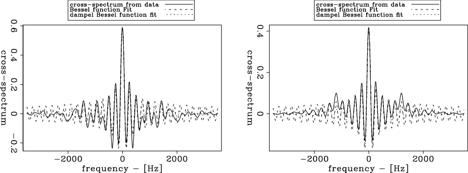
An example in which theory matches the data reasonably well is at midpoint
![]() . In Figure 8, the cross-spectrum for this midpoint and at
. In Figure 8, the cross-spectrum for this midpoint and at
![]() calculated from recording 1 and 2 are shown together with the fitted Bessel and damped Bessel functions. The estimated phase velocities and attenuation factors are
calculated from recording 1 and 2 are shown together with the fitted Bessel and damped Bessel functions. The estimated phase velocities and attenuation factors are
![]() from recording 1, and
from recording 1, and
![]() and
and
![]() ,
, ![]() from recording 2.
from recording 2.
|
|---|
|
bessels
Figure 8. Cross-spectrum at |
|
|
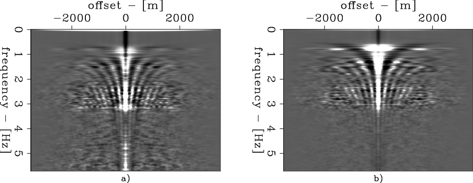
This analysis is performed for all frequencies and on both recordings. The cross-spectrum calculated at midpoint
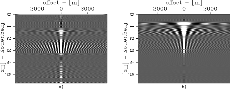
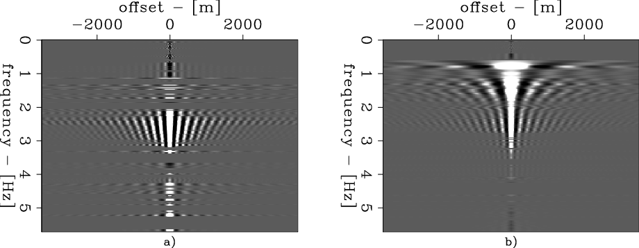
![]() for all frequencies from recording 1 and 2 are shown in Figure 9. The best fit of Bessel functions to the midpoint-gathers in Figure 9 are shown in Figure 10 and the best fit of damped Bessel functions to the midpoint gathers in Figure 10 are shown in Figure 11. The estimated dispersion curves and attenuation factors for the midpoint gather at
for all frequencies from recording 1 and 2 are shown in Figure 9. The best fit of Bessel functions to the midpoint-gathers in Figure 9 are shown in Figure 10 and the best fit of damped Bessel functions to the midpoint gathers in Figure 10 are shown in Figure 11. The estimated dispersion curves and attenuation factors for the midpoint gather at
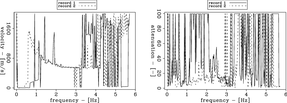
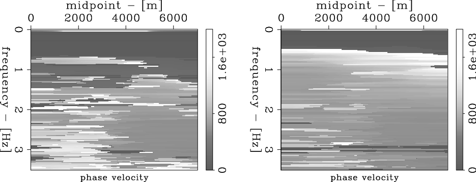
![]() are shown in Figure 12. The dispersion curves estimated for all midpoints from recording 1 and 2 are shown together in Figure 13. The dispersion curves range from values twice as large as the estimated group velocity of
are shown in Figure 12. The dispersion curves estimated for all midpoints from recording 1 and 2 are shown together in Figure 13. The dispersion curves range from values twice as large as the estimated group velocity of
![]() to velocities slightly smaller than the estimated group velocity. Although there are some spurious estimated phase velocities, a clear trend can be seen towards the right side of the array for generally higher phase velocities. The estimated attenuation coefficients vary much more strongly and become seemingly more incoherent with frequency. For the midpoint gather at
to velocities slightly smaller than the estimated group velocity. Although there are some spurious estimated phase velocities, a clear trend can be seen towards the right side of the array for generally higher phase velocities. The estimated attenuation coefficients vary much more strongly and become seemingly more incoherent with frequency. For the midpoint gather at
![]() and the frequency band of 1 to 3 Hz, the attenuation factor seems to be in the range of
and the frequency band of 1 to 3 Hz, the attenuation factor seems to be in the range of ![]() to
to ![]() .
.
|
|---|
|
spacm375o
Figure 9. Cross-spectra calculated from recording 1, in a) and 2 in b) at |
|
|
|
|---|
|
spacm375f
Figure 10. Bessel functions fitted to the cross-spectra calculated from recording 1, in a) and 2 in b), at |
|
|
|
|---|
|
spacm375df
Figure 11. Damped Bessel functions fitted to the cross-spectra calculated from recording 1, in a) and 2 in b), at |
|
|
|
|---|
|
VQcurve
Figure 12. Dispersion curve and attenuation factors estimated from the cross-spectra at |
|
|
|
|---|
|
SPACV2d
Figure 13. Estimated phase velocity from the cross-spectra calculated along the array. A clear trend of increasing phase velocities to the right-side can be observed. [CR] |
|
|
|
|
|
|
Seismic interferometry versus spatial auto-correlation method on the regional coda of the NPE |