|
|
|
|
Seismic interferometry versus spatial auto-correlation method on the regional coda of the NPE |
Wapenaar and Fokkema (2006) derives an interferometric representation of the Green's function from energy principles. Under certain conditions, this representation can be simplified to a direct cross-correlation between two receiver stations. Consider a domain
![]() in an arbitrary, inhomogeneous medium enclosing two points
in an arbitrary, inhomogeneous medium enclosing two points
![]() and
and
![]() , bounded by an arbitrarily shaped surface
, bounded by an arbitrarily shaped surface
![]() with outward pointing normal vector
with outward pointing normal vector
![]() . The interferometric representation of the Green's function for the vertical component of particle velocity measured at
. The interferometric representation of the Green's function for the vertical component of particle velocity measured at
![]() in response to a vertical force-impulse point-source acting at
in response to a vertical force-impulse point-source acting at
![]() is given in the frequency-domain as follows (Wapenaar and Fokkema, 2006):
is given in the frequency-domain as follows (Wapenaar and Fokkema, 2006):
 denotes angular frequency. The notation convention for Green's functions is that superscripts denote the receiver (first) and source type (second), and subscripts denote the components of the source (first) and receiver (second) fields. The fields and sources in the elastodynamic system are particle velocity
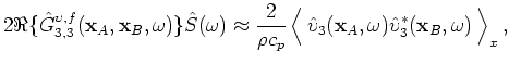
The interferometric integral in equation 1 represents the real part of the elastodynamic Green's function between two receiver stations located at A and B, as a summation of cross-correlations of independent measurements at the two receiver stations. (Independent measurements of responses of various source components and types located on a surface enclosing both receivers are required to evaluate this integral.) The integral can be modified to reflect the field configuration of the NPE, where the receivers are located just below the traction-free surface, that has
![]() . The domain integral is split into two segments,
. The domain integral is split into two segments,
![]() and
and
![]() , which are the parts of the domain boundary that coincide with the traction-free surface and the remainder, respectively. Thus the interferometric representation, equation 1, can be split into two parts:
, which are the parts of the domain boundary that coincide with the traction-free surface and the remainder, respectively. Thus the interferometric representation, equation 1, can be split into two parts:
 at the traction-free surface satisfies
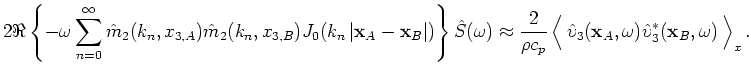
Following Wapenaar and Fokkema (2006), consider the situation when the medium outside
![]() is homogeneous and when the wavefield is generated by many mutually uncorrelated sources located on
is homogeneous and when the wavefield is generated by many mutually uncorrelated sources located on
![]() , acting simultaneously with a weighted power spectrum,
, acting simultaneously with a weighted power spectrum,
![]() . The integral over
. The integral over
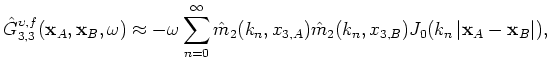
![]() in equation 2, can be evaluated by a direct cross-correlation between recordings of particle velocity at receiver stations A and B:
in equation 2, can be evaluated by a direct cross-correlation between recordings of particle velocity at receiver stations A and B:
 is the P-wave velocity. Note that the weighting factor
A similar situation occurs for earthquake tremor. Aki Aki (1957) developed a technique named the spatial auto-correlation method. The close relationship between SI and SPAC was reported by Yokoi and Margaryan (2008). Their steps are briefly repeated here to derive from equation 3 a relationship used in the SPAC method. For a wavefield dominated by the surface modes, the frequency-domain Green's function for the vertical component of particle velocity measured at
![]() in response to a vertical force-impulse point-source acting at
in response to a vertical force-impulse point-source acting at
![]() is
is
 is a normalized eigenfunction, and
 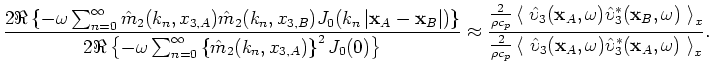 ), the higher-order terms can be neglected, and equation 6 simplifies to
 is defined as the azimuthally averaged auto-correlation coefficient. The wavenumber of the fundamental surface-wave mode is given by a specific dispersion curve,
Notice from equation 7 how the cross-spectra in frequency and space are predicted to obey Bessel functions, with oscillations determined by the phase velocity. The Bessel function of the first kind is real-valued. The cross-spectrum on the right hand-side is complex-valued, but if the conditions that lead to equation 7 are fulfilled, the imaginary component vanishes (Asten, 2006), (
![]() is always real). The real part of the cross-spectrum is retrieved as the zero-lag temporal cross-correlation, i.e., a spatial auto-correlation coefficient. It should be noted that the close relationship between SI and SPAC seems to hold only for surface-waves in horizontally stratified media. The SPAC method as commonly applied involves fitting Bessel functions to the computed auto-correlation coefficient with frequency, with explicit directional averaging of the wavefield in all directions. In the case of isotropic wavefields, this averaging is unnecessary (Aki, 1957; Okada, 2003). The coda of the NPE quickly becomes isotropic after the first break, thus this relationship seems suitable for the cross-spectra calculated from NPE data. To introduce an estimation of attenuation, the Green's function, equation 4, is supplemented with an exponential attenuation factor
is always real). The real part of the cross-spectrum is retrieved as the zero-lag temporal cross-correlation, i.e., a spatial auto-correlation coefficient. It should be noted that the close relationship between SI and SPAC seems to hold only for surface-waves in horizontally stratified media. The SPAC method as commonly applied involves fitting Bessel functions to the computed auto-correlation coefficient with frequency, with explicit directional averaging of the wavefield in all directions. In the case of isotropic wavefields, this averaging is unnecessary (Aki, 1957; Okada, 2003). The coda of the NPE quickly becomes isotropic after the first break, thus this relationship seems suitable for the cross-spectra calculated from NPE data. To introduce an estimation of attenuation, the Green's function, equation 4, is supplemented with an exponential attenuation factor ![]() , (Aki and Richards, 2002). The final model for the frequency-domain spatial auto-correlation coefficient
becomes
, (Aki and Richards, 2002). The final model for the frequency-domain spatial auto-correlation coefficient
becomes
|
|
|
|
Seismic interferometry versus spatial auto-correlation method on the regional coda of the NPE |
![$\displaystyle - \oint_{\partial\mathbf{D}_0} \left[ \hat{G}_{3,i3}^{\upsilon,h}...
...athbf{x},\omega) \right\}^*\right] \mathrm{d}^2\mathbf{x} \hspace{.25cm}\notag,$](img26.png)