Angle-domain common-image gathers in generalized coordinates

Polar coordinates

The polar coordinate system (see Figure 3b), where the extrapolation direction is oriented along the radial direction, is appropriate for generating 2D Green's function estimates. The polar coordinate system is defined by

$$\left[ \begin{array}{c} x_1\\ x_3 \end{array} \right] = \left[ \... ... {\rm cos} \xi_1 \\ a \xi_3 {\rm sin} \xi_1 \\ \end{array} \right].$$ (17)

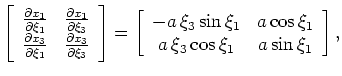
The partial derivative transformation matrix is

$$\left[ \begin{array}{cc} \frac{\partial x_1}{\partial \xi_1}& \fr... ...\ a \xi_3 {\rm cos} \xi_1 & a {\rm sin} \xi_1 \end{array}\right],$$ (18)

which leads to the following ADCIG equation:

$$- \left. \frac{\partial \xi_3}{\partial h_{\xi_1}}\right\vert _{\... ...\rm cos} \xi_1 {\rm sin} ,\alpha \right) } = - \xi_3 {\rm tan} \gamma.$$ (19)

Thus, one cannot calculate ADCIGs directly with Fourier-based methods in polar coordinates because of the spatial geometric dependence on $\xi_3$. However, polar-coordinate ADCIGs can be calculated using slant-stack operators (, ), because the geometric factor $\xi_3$ is no more than a local weight applied to the velocity model used to calculate the angle gathers.

Angle-domain common-image gathers in generalized coordinates