next up previous [pdf]

Next: Gold codes Up: Phase encoding with Gold Previous: Introduction

Prestack exploding-reflector modeling

Starting from a prestack image obtained by wave-equation migration represented by a single SODCIG, areal source and receiver wavefields are modeled at the surface by

\begin{displaymath}\begin{array}{cc} S(x,y,z=0,\omega;{\bf x}_m) = G({\bf x}_m-{...
... h};x,y,z=0,\omega)*I_r({\bf x},{\bf h};{\bf x}_m), \end{array}\end{displaymath} (A-1)

where $ S(x,y,z=0,\omega;{\bf x}_m)$ 
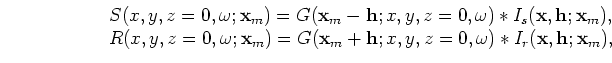
is the source wavefield and $ R(x,y,z=0,\omega;{\bf x}_m)$ is the receiver wavefield. $ I_s({\bf x},{\bf h};{\bf x}_m)$ and $ I_r({\bf x},{\bf h};{\bf x}_m)$ are the prestack images used as initial conditions for the source and receiver wavefield extrapolation, respectively, at a selected position, $ {\bf x}_m$. These prestack images should be dip-independent gathers. They are computed by re-mapping the dip along the offset direction according to the apparent geological dip (Biondi, 2007). $ G({\bf x}_m\pm{\bf h};x,z=0,\omega)$ represents the operator that extrapolates the wavefields from the subsurface to the surface; $ {\bf h}$ is the subsurface offset; $ \omega$ is the temporal frequency; and $ {\bf x}$ is the vector of spatial coordinates.

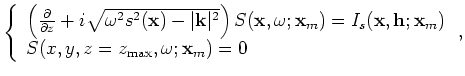
In the case of using an one-way extrapolator, the source and receiver wavefields are upward continued according to the one-way wave equations
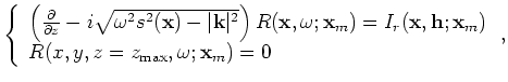
$\displaystyle \left\{ \begin{array}{l}
\left( \frac{\partial}{\partial z}+i\sqr...
...};{\bf x}_m) \\
S(x,y,z=z_{\rm max},\omega;{\bf x}_m) = 0 \end{array} \right.,$     (A-2)

and
$\displaystyle \left\{ \begin{array}{l}
\left( \frac{\partial}{\partial z}-i\sqr...
...};{\bf x}_m) \\
R(x,y,z=z_{\rm max},\omega;{\bf x}_m) = 0 \end{array} \right.,$     (A-3)

where $ s({\bf x})$ is the slowness at $ {\bf x}$; $ {\bf k}=(k_x,k_y)$ is the spatial wavenumber vector.

Using the linearity of the wave propagation, sets of individual modeling experiments can be combined into the same areal data, such that the amount of data input into migration can be significantly decreased, reducing its cost. However, this procedure generates crosstalk when applying the imaging condition during migration.

Guerra and Biondi (2008) introduce strategies to attenuate the crosstalk. Migration of $ ({\bf x},\omega)$-random-phase encoded data disperses the crosstalk energy throughout the image as a pseudo-random background noise. By adding more realizations of random-phase encoded areal data, the speckled noise can be further attenuated. The encoded source wavefield, $ {\widetilde S}({\bf x},{\bf p}_m,\omega)$, and the encoded receiver wavefield, $ {\widetilde R}({\bf x},{\bf p}_m,\omega)$, are synthesized according to

$\displaystyle \left\{ \begin{array}{l}
\left( \frac{\partial}{\partial z}+i\sqr...
...\\
{\widetilde S}(x,y,z=z_{\rm max},{\bf p}_m,\omega) = 0 \end{array} \right.,$     (A-4)

and
$\displaystyle \left\{ \begin{array}{l}
\left( \frac{\partial}{\partial z}-i\sqr...
...\\
{\widetilde R}(x,y,z=z_{\rm max},{\bf p}_m,\omega) = 0 \end{array} \right.,$     (A-5)

where $ \widetilde{I}_s({\bf x},{\bf h},{\bf p}_m,\omega)$ and $ \widetilde{I}_r({\bf x},{\bf h},{\bf p}_m,\omega)$ are the encoded SODCIGs after rotations. They are defined as follows:
$\displaystyle \widetilde{I}_s({\bf x},{\bf h},{\bf p}_m,\omega)$ $\displaystyle =$ $\displaystyle \sum_{{\bf x}_m}I_s({\bf x},{\bf h},{\bf x}_m)\beta({\bf x},{\bf x}_m,{\bf p}_m,\omega),$ (A-6)
$\displaystyle \widetilde{I}_r({\bf x},{\bf h},{\bf p}_m,\omega)$ $\displaystyle =$ $\displaystyle \sum_{{\bf x}_m}I_r({\bf x},{\bf h},{\bf x}_m)\beta({\bf x},{\bf x}_m,{\bf p}_m,\omega),$ (A-7)

where $ \beta({\bf x},{\bf x}_m,{\bf p}_m,\omega)=e^{i\gamma({\bf x},{\bf x}_m,{\bf p}_m,\omega)}$ is the phase-encoding function; the variable $ {\bf p}_m$ is the index of different realizations of phase encoding.

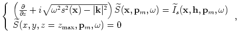
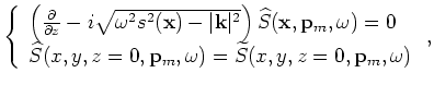
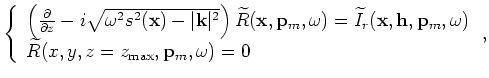
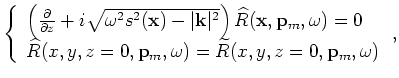
The areal shot migration is performed by downward continuation of the areal source and receiver wavefields according to the following one-way wave equations
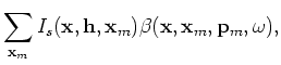
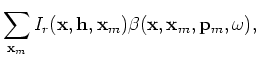
$\displaystyle \left\{ \begin{array}{l}
\left( \frac{\partial}{\partial z}-i\sqr...
...bf p}_m,\omega) = {\widetilde S}(x,y,z=0,{\bf p}_m,\omega) \end{array} \right.,$     (A-8)

and
$\displaystyle \left\{ \begin{array}{l}
\left( \frac{\partial}{\partial z}+i\sqr...
...bf p}_m,\omega) = {\widetilde R}(x,y,z=0,{\bf p}_m,\omega) \end{array} \right.,$     (A-9)

where the encoded source wavefield, $ {\widetilde S}({\bf x},{\bf p}_m,\omega)$, and the encoded receiver wavefield, $ {\widetilde R}({\bf x},{\bf p}_m,\omega)$, are used as boundary conditions.

The image, $ \widehat{I}({\bf x},{\bf h})$, is obtained by cross-correlation of the source wavefield, $ {\widehat S}({\bf x},{\bf p}_m,\omega)$, with the receiver wavefield, $ {\widehat R}({\bf x},{\bf p}_m,\omega)$

$\displaystyle \widehat{I}({\bf x},{\bf h}) = \sum_{\omega} \sum_{{\bf p}_m} \wi...
...\bf x}-{\bf h},{\bf p}_m,\omega) \widehat{R}({\bf x}+{\bf h},{\bf p}_m,\omega),$ (A-10)

where $ ^{\star}$ 
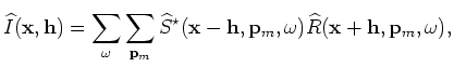
represents complex conjugation.


next up previous [pdf]

Next: Gold codes Up: Phase encoding with Gold Previous: Introduction

2009-04-13