|
|
|
|
Exact seismic velocities for TI media and extended Thomsen formulas for stronger anisotropies |
Thomsen's weak anisotropy formulation (Thomsen, 1986), being a collection of approximations
designed specifically for use in velocity analysis for exploration geophysics,
is clearly not exact. Approximations incorporated into the formulas
become most apparent for angles ![]() greater than about 15
greater than about 15![]() from the vertical,
especially for compressional and vertically polarized shear wave velocities
from the vertical,
especially for compressional and vertically polarized shear wave velocities
![]() and
and
![]() , respectively. For VTI media, angle
, respectively. For VTI media, angle ![]() is
measured from the
is
measured from the ![]() -vector pointing directly into the earth.
-vector pointing directly into the earth.
For reference purposes, I include here the exact velocity formulas for;
quasi-P, quasi-SV, and SH seismic waves at all angles in a VTI elastic medium.
These results are available in many places
(Postma, 1955; Musgrave, 1959, 2003; Rüger, 2002; Thomsen, 2002),
but were taken directly from Berryman (1979)
with only some minor changes of notation; specifically, the ![]() ,
,![]() ,
,![]() ,
,![]() ,
,![]() ,
,![]() notation for stiffnesses
has been translated to the Voigt
notation for stiffnesses
has been translated to the Voigt ![]() stiffness notation wherein
stiffness notation wherein ![]() ,
, ![]() ,
,
![]() ,
, ![]() ,
, ![]() , and
, and ![]() . The results are:
. The results are:
For VTI symmetry, the stiffness matrix ![]() is defined for
is defined for
![]() by
by
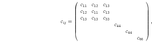 .
In an isotropic system (which is a more restrictive case than our current
interests),
.
In an isotropic system (which is a more restrictive case than our current
interests),
Expressions for phase velocities in Thomsen's weak anisotropy
limit can be found in many places, including Thomsen (1986, 2002)
and Rüger (2002).
The pertinent expressions for phase velocities in VTI media
as a function of angle ![]() ,
measured as previously mentioned from the vertical direction, are
,
measured as previously mentioned from the vertical direction, are
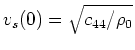 , where
 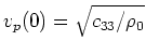 ,
,  is a measure of the shear wave anisotropy and birefringence.
Parameter
is a measure of the shear wave anisotropy and birefringence.
Parameter
All three of these parameters , ![]() ,
, ![]() can play important
roles in the velocities given by equations 7-9
when the anisotropy is large, as would be the case in fractured reservoirs when the
crack densities are high enough. If crack densities are very low, then the SV shear wave will
actually have no dependence on angle of wave propagation. Note that the
so-called anellipticity parameter (Dellinger et al., 1993; Fomel, 2004; Tsvankin, 2005, p. 253),
can play important
roles in the velocities given by equations 7-9
when the anisotropy is large, as would be the case in fractured reservoirs when the
crack densities are high enough. If crack densities are very low, then the SV shear wave will
actually have no dependence on angle of wave propagation. Note that the
so-called anellipticity parameter (Dellinger et al., 1993; Fomel, 2004; Tsvankin, 2005, p. 253),
![]() , vanishes when
, vanishes when
![]() --
which (as will be shown) does happen to a very good approximation for low crack densities.
Then, the results are anisotropic but have the special (elliptical) shape to the wave front
mentioned previously.
--
which (as will be shown) does happen to a very good approximation for low crack densities.
Then, the results are anisotropic but have the special (elliptical) shape to the wave front
mentioned previously.
For each of these phase velocities, the derivation of Thomsen's approximation has
included a step that removes the square on the left-hand side of equations
1, 2, and 4 --
obtained by expanding a square root of the right hand side. This step introduces a
factor of ![]() multiplying the
multiplying the ![]() terms on the right
hand side, and -- for example -- immediately explains how equation 8
is obtained from equation 4. The other two equations for
terms on the right
hand side, and -- for example -- immediately explains how equation 8
is obtained from equation 4. The other two equations for ![]() and
and
![]() , i.e.,
equations 7 and 8,
involve additional approximations. More of the details about the nature of these
approximations are elucidated by first obtaining an alternative approximate formulation.
, i.e.,
equations 7 and 8,
involve additional approximations. More of the details about the nature of these
approximations are elucidated by first obtaining an alternative approximate formulation.
|
|
|
|
Exact seismic velocities for TI media and extended Thomsen formulas for stronger anisotropies |