Exact seismic velocities for TI media and extended Thomsen formulas for stronger anisotropies

APPENDIX B: HTI FORMULAS FROM VTI FORMULAS

Probably the easiest way to obtain formulas pertinent to HTI (horizontal transverse isotropy) from VTI (vertical transverse isotropy) is to leave the stiffness matrix $c_{ij}$ alone, and simply reinterpret the meaning of the Cartesian indices $i,j$. For VTI media, one typical choice is $x_3 = z$, where $\hat{z}$ is the vertical direction at the surface of the earth, or more often the direction down into the earth. Then, the angle of incidence $\theta$ is measured with respect to $\hat{z}$, where $\theta = 0$ means parallel to $\hat{z}$ and pointing into the earth, and $\theta = \pi/2$ means horizontal incidence.

Considering aligned vertical fractures, with their axes of symmetry in the direction $x \equiv x_3$, the matrix $c_{ij}$ itself presented in the main text need not change, but the meaning of the angles does change. Clearly, the simplest case to study -- and the only one analyzed here -- is the case of waves propagating at some angle to vertical but always having a component in the direction $x_3 = x$, while also having $x_2 = y = 0$, thus lying in the $xz$-plane perpendicular to the fracture plane. (This case is special, but all other wave speeds at other angles of propagation are easily found as a linear combination -- depending specifically on the azimuthal angle $phi$ at the earth surface -- of these values and those in the plane of the fractures themselves.) Then,

$$\theta^H + \theta^V = \frac{\pi}{2},$$ (B-1)

where $\theta^V$ corresponds exactly to the $\theta$ appearing in all the formulas up to equation 39 in the main text, and $\theta^H$ is the effective angle in the $xz$-plane of incidence under consideration, i.e., the one perpendicular to the vertical fractures in the reservoir. To obtain wave speeds at the angle $\theta^H$, just substitute $\theta \equiv \theta^V = \frac{\pi}{2} - \theta^H$, or write the speeds as

$$^Hv_p^2(\theta^H) \equiv v_p^2(\theta^V) = v_p^2(\frac{\pi}{2}- \theta^H),$$ (B-2)

$$^Hv_{sv}^2(\theta^H) \equiv v_{sv}^2(\theta^V) = v_p^2(\frac{\pi}{2}- \theta^H),$$ (B-3)

and

$$^Hv_{sh}^2(\theta^H) \equiv v_{sh}^2(\theta^V) = v_p^2(\frac{\pi}{2}- \theta^H).$$ (B-4)

Since all the angular dependence in the exact formulas is in the form of $\sin^2\theta$ and $\cos^2\theta$, and since $\sin^2(\frac{\pi}{2}-\theta) = \cos^2\theta$ and vice versa, the entire procedure amounts to switching the locations of $\sin^2\theta$ and $\cos^2\theta$ with $\cos^2\theta^H$ and $\sin^2\theta^H$ everywhere in the exact expressions.

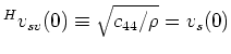
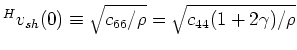
This procedure is obviously very straightforward to implement. The final results analogous to Thomsen's formulas are:

$$^Hv_p(\theta^H)/^Hv_p(0) \simeq 1 - \frac{\epsilon}{1+2\epsi... ...2\theta^H\cos^2\theta^H}{[1 - \cos2\theta^H\cos2\theta_m^H]},$$ (B-5)

$$^Hv_{sv}(\theta^H)/^Hv_{sv}(0) \simeq 1 + \left[c_{33}/c_{44... ...2\theta^H\cos^2\theta^H}{[1 - \cos2\theta^H\cos2\theta_m^H]}.$$ (B-6)

and

$$^Hv_{sh}(\theta^H)/^Hv_{sh}(0) \simeq 1 - \frac{\gamma}{1+2\gamma}\sin^2\theta^H.$$ (B-7)

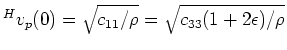And the $\theta^H = 0$ velocities are: $^Hv_p(0) = \sqrt{c_{11}/\rho} = \sqrt{c_{33}(1+2\epsilon)/\rho}$, $^Hv_{sv}(0) \equiv \sqrt{c_{44}/\rho} = v_s(0)$, and $^Hv_{sh}(0) \equiv \sqrt{c_{66}/\rho} = \sqrt{c_{44}(1+2\gamma)/\rho}$. Also, recall that $\cos^2\theta_m^H = \sin^2\theta_m^V$.

For azimuthal angles $\phi \ne \pm\frac{\pi}{2}$, the algorithm for computing the wave speeds is to replace $\sin^2 \theta^V$ by $\cos^2\theta^H\sin^2 \phi$ and $\cos^2\theta^V = 1 - \sin^2\theta^V$ by $1 - \cos^2\theta^H\sin^2\phi$ in the exact formulas, and corresponding replacements in the approximate ones. Then, there is no angular dependence when $\phi = 0$ or $\pi$ as our point of view then lies within the plane of the fracture itself. And, when $\phi = \pm\frac{\pi}{2}$, the above stated results for the $xz$-plane hold.

Wave equation reciprocity guarantees that the polarizations of the various waves are of the same types as our mental translation from VTI media to HTI media is made.

It is also worth pointing out that the labels $SH$ and $SV$ for the shear waves -- although analogous -- are, however, surely not strictly valid for the HTI case. For VTI media, the quasi-$SH$-wave really does have horizontal polarization at least at $\theta = 0$ and $\pi/2$, whereas the corresponding wave for HTI media, instead has polarization parallel ($\parallel$) to the fracture plane. For VTI media, the so-called quasi-$SV$-wave has its polarization in the plane of propagation, but this polarization direction is only truly vertical for $\theta = \pm \frac{\pi}{2}$, at which point its polarization is both vertical and perpendicular to the horizontal plane of symmetry. The corresponding situation for HTI media has the wave corresponding to the $SV$-wave with polarization again in the plane of propagation, but this is actually only vertical at $\theta^H = \frac{\pi}{2}$, and also parallel to the fracture plane; however, for all other angles its polarization has a component that is perpendicular ($\perp$) to the plane of the fractures. So a much more physically accurate naming convention for these waves would make use of the following designations:

$$^Hv_{sh}(\theta^H) \to ^Hv_{s\parallel}(\theta^H),$$ (B-8)

for the HTI wave corresponding to the quasi-SH-wave in the VTI case, and

$$^Hv_{sv}(\theta^H) \to ^Hv_{s\perp}(\theta^H),$$ (B-9)

for the HTI wave corresponding to the quasi-SV-wave in the VTI case. Although this notation is hereby being recommended, it will actually not be used in the main text as the current choices (as well as the various caveats) will no doubt be sufficiently familiar to most readers that it is probably not be essential to make this change in the present paper. In closing, also note that Thomsen (2002) uses the same $\parallel$ and $\perp$ notation for very similar purposes.

Exact seismic velocities for TI media and extended Thomsen formulas for stronger anisotropies