Plane-wave migration in tilted coordinates

BP 2004 velocity benchmark dataset

The BP 2004 velocity benchmark dataset is designed to test velocity estimation. Figure 11 shows the velocity model of the dataset. One of the challenges for velocity analysis of this dataset is the delineation of the two salt bodies. The salt body on the left, modeled after a salt body in the Gulf of Mexico, is a complex, multi-valued salt body with a greatly rugose top. Some parts of its top, flanks and the sediment intrusion inside the salt are steeply dipping. It is difficult for downward continuation migration to image these features. The salt body on the right, modeled after a salt body in the western Africa, is deeply rooted, and its roots are very steep. Overturned and prismatic waves play a key role in imaging the two roots of the right salt body. Downward continuation loses the overturned energy and cannot connect these two roots. Even with the true velocity, it is challenging to image these complex salt bodies.

We run both plane-wave migrations in tilted coordinates and downward continuation migration for comparison. Two hundred plane-wave sources are generated in total, and the take-off angles at the surface range from $-45^\circ$ to $45^\circ$. No attempt is made to attenuate multiples, thus the images are contaminated by the multiples. The $80^\circ$ finite-difference one-way extrapolator (Lee and Suh, 1985) is applied for both migrations.

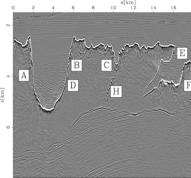
Figure 12 shows the velocity model of the left salt body. Figure 13 and Figure 14 compare the images from the two migrations. Notice that remarks A, B, C, D, E, F, G and H in Figures 12, 13 and 14 are in exactly the same locations. Figures 13 and 14 are the images obtained by plane-wave migration in tilted coordinates and downward continuation migration, respectively. In both figures, the bottom of the big salt canyon is well imaged. But the steep flanks of the canyon at A and B, which are absent in Figure 14, are correctly imaged in Figure 13. This is also true for the small salt canyon at C. Although the salt canyon flank at D is imaged by downward continuation migration in Figure 14, it is not positioned correctly due to the limited accuracy of the operator compared to the model (Figure 12). The rugose top of the salt in Figure 13 is more continuous than that in Figure 14. The steep salt flanks in the multi-valued part at E, F and G and the sediment intrusion below the small salt canyon at H are greatly improved in Figure 13 by plane-wave migration in tilted coordinates, because they are illuminated by overturned or high-angle energy, which cannot be handled by downward continuation migration.

bpleftvel
Figure 12. The velocity model of the left salt body.

bpleftsalttilt
Figure 13. The images of the left salt body obtained by plane-wave migration in tilted coordinates.

bpleftsaltnotilt
Figure 14. The images of the left salt body obtained by downward continuation migration.

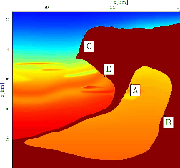
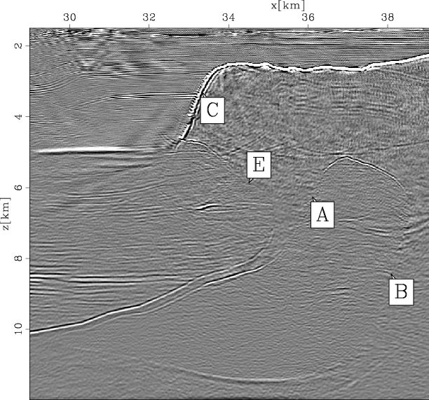
Figure 15 shows the velocity model of salt body on the right. Figure 16 and Figure 17 compare the images from the two migrations. Notice that remarks A, B, C, D and E in Figures 15, 16 and 17 are in exactly the same locations. Figure 16 is obtained by plane-wave migration in tilted coordinates, and Figure 17 is obtained by downward continuation migration. The top of the salt and sediments inside the salt are well imaged in both figures. But the salt flanks at A, B and D that are illuminated by the overturned or high-angle energy in vertical Cartesian coordinates are absent in Figure 17. In contrast, this overturned energy is handled by plane-wave migration in tilted coordinates, producing a good image of the flanks of the salt roots. In Figure 17, we can see the steep flank at C, but it is not correctly positioned compared to Figure 16 because of the limited accuracy of the wavefield extrapolator. Note that the salt flank at E is absent in both images. This flank is illuminated mainly by prismatic waves which bounce off the salt root below E. The propagation direction of the prismatic waves varies greatly before and after the bounce at the salt boundary, and it is difficult to model them accurately in one coordinate system.

bprightvel
Figure 15. The velocity model of the right salt body.

bprightsalttilt
Figure 16. The images of the right salt body obtained by plane-wave migration in tilted coordinates.

bprightsaltnotilt
Figure 17. The images of the right salt body obtained by downward continuation migration.

Figures 13, 14, 16 and 17 show that plane-wave migration in tilted coordinates can handle overturned and high-angle energy and delineate complex salt bodies much better than downward continuation migration.

Plane-wave migration in tilted coordinates