Plane-wave migration in tilted coordinates

One-way wave equation migration

Surface seismic data are usually recorded as shot gathers. Each shot gather represents a point-source exploding experiment. The most straightforward way to obtain the subsurface image of the earth is shot-profile migration, in which we obtain the local image of each experiment by migrating each shot gather independently and form the whole image of the subsurface by stacking all the local images. Migrating one shot gather using a typical shot-profile migration algorithm includes two steps. First, source and receiver wavefields are extrapolated from the surface to all depths in the subsurface. Second, the images are constructed by cross-correlating the source and receiver wavefields.

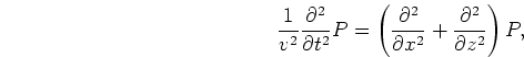
The propagation of waves in the subsurface is approximately governed by a two-way acoustic wave equation. In an isotropic medium, it is defined as follows:

$$\frac{1}{v^2}\frac{\partial^2}{\partial t^2}P=\left( \frac{... ...al^2 }{\partial x^2}+\frac{\partial^2}{\partial z^2}\right)P,$$ (1)

where $P=P(x,z,t)$ is the pressure field and $v=v(x,z)$ is the velocity of the medium. To reduce computational costs, we usually use the one-way instead of two-way wave equations for wavefield extrapolation:

$$\frac{\partial }{\partial z}S= -\frac{i\omega}{v}\sqrt{1+\left(\frac{v}{\omega}\frac{\partial}{\partial x}\right)^2}S,$$ (2)

$$\frac{\partial }{\partial z}R= +\frac{i\omega}{v}\sqrt{1+\left(\frac{v}{\omega}\frac{\partial}{\partial x}\right)^2}R,$$ (3)

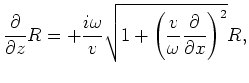for wavefield extrapolation, where $\omega$ is angular frequency, $S=S(s_x,x,z,\omega)$ is the source wavefield, $R=R(s_x,x,z,\omega)$ is the receiver wavefield, and $s_x$ is the source location. Given the propagation direction of the source and receiver wavefields, we use the down-going one-way wave equation (equation 2) for the source wavefield and the up-going one-way wave equation (equation 3) for the receiver wavefield. Both are obtained by splitting the two-way acoustic equation (Zhang, 1993). After the wavefield extrapolation, we have the source and receiver wavefields at all depths and the image is constructed by cross-correlating the source and receiver wavefields as follows:

$$I_{s_x}=\int S^*(s_x,x,z,\omega)R(s_x,x,z,\omega)d\omega ,$$ (4)

where $S^*$ is the complex conjugate of the source wavefield $S$. Finally the whole image is generated by stacking the images of all the shots as follows:

$$I=\int I_{s_x} d{s_x}.$$ (5)

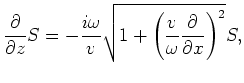
If there is no lateral velocity variation, equations 2 and 3 can be solved by the phase-shift method in the frequency-wavenumber domain with accuracy up to $90^\circ$. Otherwise, an approximation for the square root operator has to be made to solve equations 2 and 3 numerically. The accuracy of a wavefield extrapolator determines the maximum angle between the propagation direction and the vertical direction that can be modeled accurately. most algorithms can model waves that propagate almost vertically downward. For example, the classic $15^\circ$ equation (Claerbout, 1971) can handle waves propagating $15^\circ$ from the vertical direction. However, most algorithms cannot model waves propagating almost horizontally in a medium with strong lateral variation. Finite-difference methods handle lateral variation of the media well, but the cost of improving the accuracy at high angles is high. Hybrid algorithms such as Fourier finite-difference take advantage of both the finite-difference and phase-shift methods. When the lateral variation of the medium is mild, phase-shift plays the important role and can achieve good accuracy. The finite-difference part becomes more important where the actual velocity value is far from the reference velocity, but again is difficult to propagate high-angle energy accurately with a reasonable cost. It is difficult to solve the one-way wave equation accurately to model high-angle energy in a medium with strong lateral variation.

One-way wave equations also function as dip filters. During the source wavefield extrapolation, only the down-going energy is permitted using the down-going one-way wave equation; up-going energy is filtered out. Similarly, the down-going energy is filtered out during the receiver wavefield extrapolation. Therefore, overturned energy is filtered out in both source and receiver wavefields in conventional downward continuation migration.

Conventional downward continuation migration is not sufficient for imaging steeply dipping reflectors, since they are mainly illuminated by high-angle and overturned energy. These are the two main migration issues that we attempt to resolve with plane-wave migration in tilted coordinates.

Plane-wave migration in tilted coordinates