Angle-domain parameters computed via weighted slant-stack

Transformation of the Main diagonal

Figures 4 and 5 show that, for ADCIGs at CMP coordinates 33200 ft and 35500 ft, the energy is mainly focused at reflection angles around 0$^{\circ }$ and 40$^{\circ }$ - 50$^{\circ }$. Additionally, these figures show the original reflection-angle gather (a), the main diagonal of the Hessian transformed to the reflection-angle domain (b), and the amplitude-compensated ADCIG (c). Notice how the amplitudes are better distributed along the reflection-angle axis after compensation by the inverse of the diagonal of the Hessian. However, as only the diagonal of the Hessian is being used, the kinematic artifacts remain.

join16
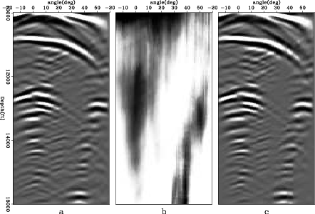
Figure 4. ADCIGs and diagonal of the transformed angle-domain Hessian at CMP coordinate 33200 ft. Before amplitude compensation (a); diagonal of the Hessian in the angle domain (b); and after amplitude compensation (c). Note the improved amplitude balance in the angle direction.

join50
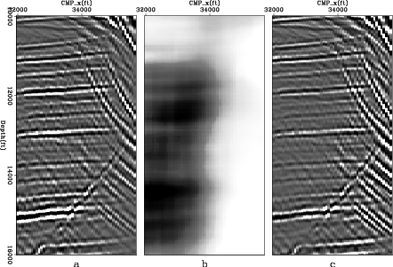
Figure 5. ADCIGs and diagonal of the transformed angle-domain Hessian at CMP coordinate 35500 ft. Before amplitude compensation (a); diagonal of the Hessian in the angle domain (b); and after amplitude compensation (c).

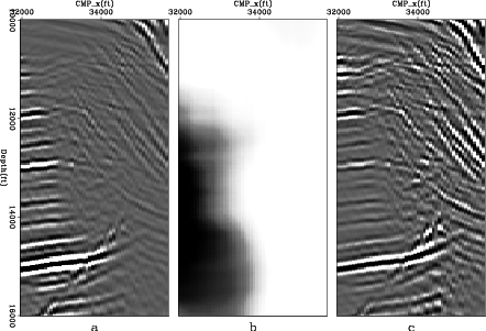
The proposed approach seems to be dependent on the amplitude strength of the events in the ADCIGs. However, as shown in the next example, it yields useful information about illumination. Figures 6, 7 and 8 show angle sections of the original angle data (a), the main diagonal of the Hessian in the angle domain (b) and the amplitude-balanced angle data (c). Again, the amplitude compensation proved to be effective. However, notice how for the zero-angle section the illumination computed in the angle domain is low at the right part of the section, in spite of the high amplitudes of the internal multiples. This confirms, to some extent, that the proposed approach can yield reliable information about illumination despite the presence of high-amplitude events not predicted in the computation of the Green's functions.

join00
Figure 6. Zero-angle section. Before amplitude compensation (a); diagonal of the Hessian in the angle domain (b); and after amplitude compensation (c). Notice the low illumination in the right part of the section, near the flank of the salt body.

join15
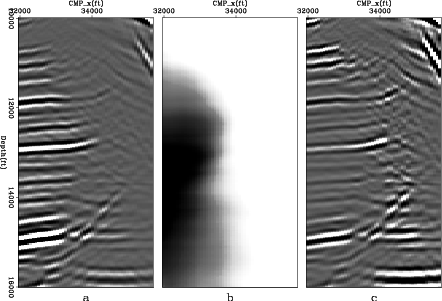
Figure 7. 15$^{\circ }$-angle section. Before amplitude compensation (a); diagonal of the Hessian in the angle domain (b); and after amplitude compensation (c). Notice the improved amplitude balance along the CMP direction.

join30
Figure 8. 30$^{\circ }$-angle section. Before amplitude compensation (a); diagonal of the Hessian in the angle domain (b); and after amplitude compensation (c).

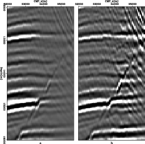
Figure 9 shows the stacked section along the angle axis, before (a) and after (b) the amplitude compensation by the inverse of the diagonal of the Hessian in the angle domain. The dimming of the amplitudes at the right portion of the section is almost eliminated. Unfortunately, however, the amplitudes of internal multiples are also increased.

Stk
Figure 9. Stack along the angle axis. Before amplitude compensation (a) and after (b).

Angle-domain parameters computed via weighted slant-stack