Target-oriented wave-equation inversion: regularization in the reflection angle

Postack comparison

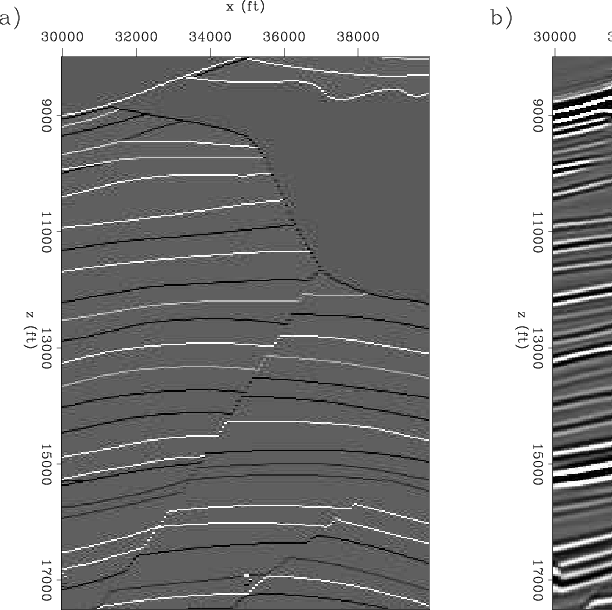
Figure 5 shows the reflection coefficients, and the zero subsurface-offset migration. The zero subsurface-offset inversion (Valenciano et al., 2006), and the stack of the inversion with regularization in the reflection angle can be seen in Figure 6. In the migration result shown in Figure 5b the reflectors dim out in the areas of low illumination (see left panel of Figure 3 for reference). In contrast, the zero subsurface-offset inversion (Figure 6a) and the stack of the inversion with regularization in the reflection angle (Figure 6b) show that: the reflectors can be followed into the shadow zones with the correct kinematics, the resolution increases, the footprint of the irregular illumination is diminished, and the faults can be followed and interpreted closer to the salt body.

It is important to remark the differences between the two inversion results in Figure 6a and Figure 6b. The inversion with regularization in the reflection angle has better defined fault planes and sediments more accurately extended into the shadow zones than the zero subsurface-offset inversion. Also, the level of noise in the zero subsurface-offset inversion is much higher. This is due to the fact that no regularization was applied in the zero subsurface-offset inversion. The regularization in the reflection angle helps to spread the image from well illuminated to poorly illuminated reflection angles, reducing the noise and eliminating non consistent artifacts.

compSisfull1
Figure 5. Target area comparison. (a) reflection coefficients, and (b) zero subsurface-offset migration.

compSisfull2
Figure 6. Target area comparison. (a) zero subsurface-offset inversion, and (b) stack of the inversion with regularization in the reflection angle (zero subsurface-offset).

The salt in the inversion images looks distorted because a residual weight designed to decrease the salt contribution was used (data values in the salt boundary are bigger than everywhere else Figure 2). This was necessary to avoid the solver expending most of the iterations decreasing the residuals in that area.

Target-oriented wave-equation inversion: regularization in the reflection angle