Target-oriented wave-equation inversion: regularization in the reflection angle

Numerical results: Sigsbee model

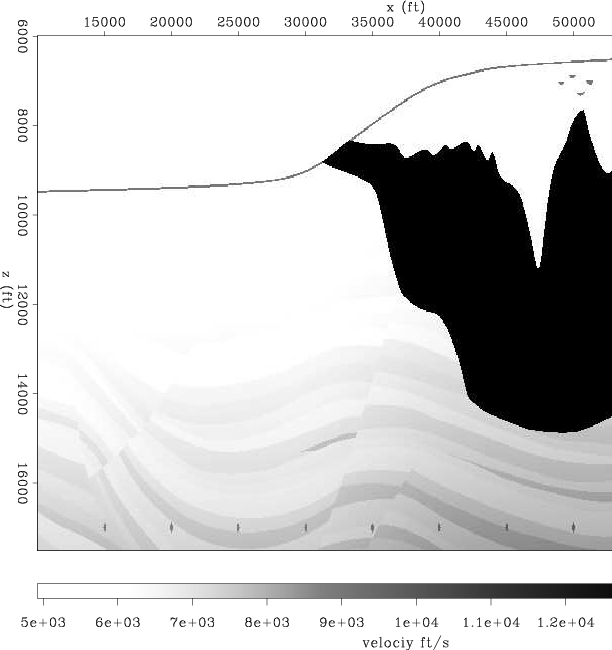
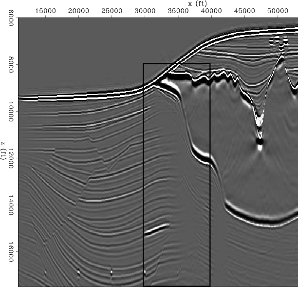
The Sigsbee data set was modeled by simulating the geological setting found on the Sigsbee escarpment in the deep-water Gulf of Mexico. The model exhibits the illumination problems due to the complex salt shape, characterized by a rugose salt top (see Figure 1). Figure 2 shows the shot-profile migration image (using cross-correlation imaging condition) corresponding to the portion of Sigsbee model shown in figure 1. Notice how the amplitudes of the reflectors fade away as they get closer to the salt.

Sisvel
Figure 1. Sigsbee stratigraphic velocity model.

migSis
Figure 2. Sigsbee shot-profile zero subsurface-offset migration image using cross-correlation imaging condition. The velocity model corresponds to Figure 1

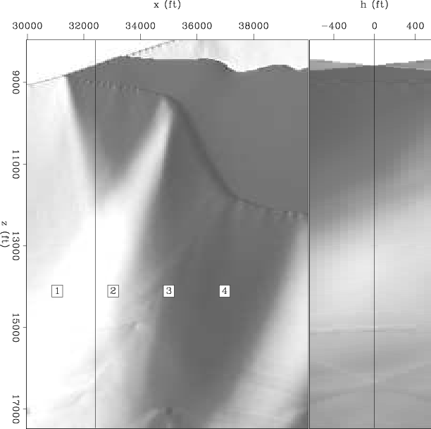
I choose a target zone close to the salt to evaluate the effects of illumination on imaging (rectangle in Figure 2). A good picture of the complexity of the focusing and defocusing of the seismic energy in this model is given by Figure 3, which shows the diagonal of the Hessian matrix in the target zone. Light gray correspond to hight amplitude and dark gray to low amplitudes. Notice how the concave and convex shape of the base of the salt, respectively, focus and defocus the seismic energy as waves propagate trough the medium.

diag
Figure 3. Diagonal of the target-oriented Hessian matrix. White correspond to hight amplitude

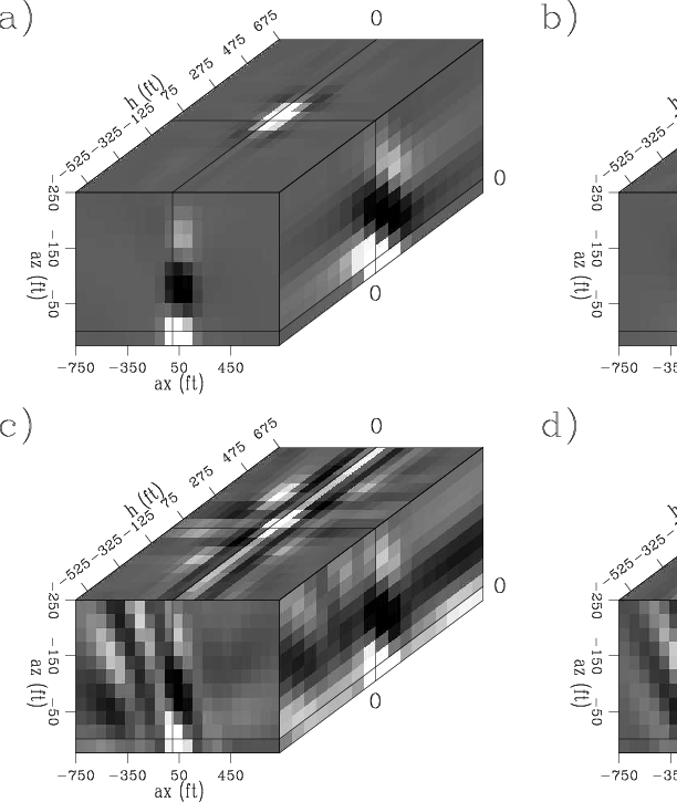
Four rows of the target-oriented Hessian matrix are shown in Figure 4. They are $11\times21\times17$ coefficient filter for constant depth and constant subsurface-offset ($h_x=0 ft$) at four different $x$ coordinates (from the sediments to the salt boundary Figure 3). Notice that only the elements of the matrix corresponding to one side of the diagonal are shown. Since the Hessian matrix is symmetric by definition half of the off diagonal terms are not computed. Figure 4a shows point 1, with coordinates ${\bf x}=(14000,31000) ft$ (far from the salt). Figure 4b shows point 2, with coordinates ${\bf x}=(14000,33000) ft$. Figure 4c shows point 3, with coordinates ${\bf x}=(14000,35000) ft$. Figure 4d shows point 4, with coordinates ${\bf x}=(14000,37000) ft$ . The shape of the filter is not dependent only on the acquisition geometry but the subsurface geometry (presence of the salt body). In the area less affected by the salt the energy is concentrated around the diagonal (center of the filter), but as we get closer to the salt, the illumination varies (in intensity and angle) and the filter behaves differently. This is due to a focusing and defocusing effect created by the salt. To correct this effect we computed the least-squares inverse image.

hesianphaseSis
Figure 4. Four rows of the target-oriented Hessian matrix, (a) point 1 ${\bf x}=(14000,31000) ft$, (b) point 2 ${\bf x}=(14000,33000) ft$, (c) point 3 ${\bf x}=(14000,35000) ft$, and (d) point 4 ${\bf x}=(14000,37000) ft$.

Target-oriented wave-equation inversion: regularization in the reflection angle