Gulf of Mexico data

I start with the Angle-Domain Common-Image Gather (ADCIG) shown in Figure 10. Panel (a) is the initial data, panel (b) the estimated multiples and panel (c) the estimated primaries.

adcig1-estimates1
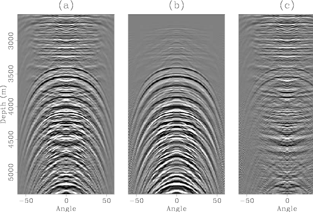
Figure 10. ADCIG from the Gulf of Mexico line of chapter 2 (a), initial estimate of the multiples (b), and the primaries (c). Note the crosstalk on both panels.

The estimate of the multiples was obtained with Radon transform in the image space presented in chapter 2 (without the apex-shift) and the estimate of the primaries was obtained simply by subtracting it from the data. Notice the residual primary energy just below 3000 m in the estimate of the primaries. Note also the residual energy from the multiples in the estimate of the primaries.

adcig1-matched-prims
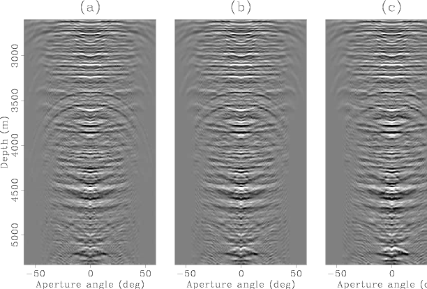
Figure 11. Estimated primaries after one (a), five (b) and ten (c) outer iterations. Notice how the residual multiples decrease with the outer iterations although are not completely eliminated.

adcig1-matched-muls
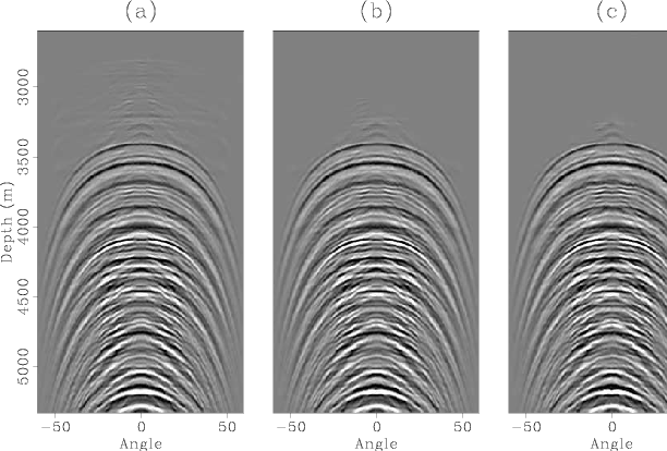
Figure 12. Estimated multiples after one (a), five (b) and ten (c) outer iterations. Here too, the residual primaries decrease and almost disappear after the 10th outer iteration.

Figure 11 shows the ADCIG after one, five and ten outer iterations. The first iteration attenuates the strongest residual multiples (compare panel (a) of Figure 11 with panel (c) of Figure 10). Subsequent iterations further reduce the residual multiples. Also, although hard to see in the hard copy, the primary energy that contaminated the estimate of multiples below 3000 m has been mapped back to the primaries. Figure 12 shows the corresponding results for the multiples. Notice again that the residual primary energy has been severely attenuated.

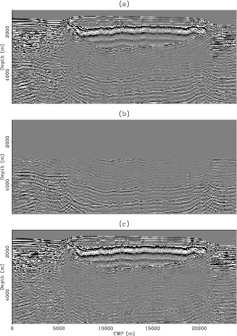
To show the impact of the better matching of the multiples in the angle stack, I applied the same steps to all the 900 ADCIGs in the seismic line. Figure 13 shows the angle stack of the data (primaries and multiples) and the angle stack of the initial estimates of the multiples and the primaries. Recall that this initial estimate of the primaries was obtained by direct subtraction of the estimate of the multiples from the data (without adaptive subtraction). All the panels are plot at the exact same clip value. Note that although most multiples have been attenuated some multiple energy remain below the salt body.

initial-stacks
Figure 13. Comparison of angle stacks for the data (panel (a)), the initial estimate of the multiples (panel (b)) and the initial estimate of the primaries (panel (c)).

In order to concentrate the comparison of the different estimates of the multiples and primaries to the region where the multiples are present, I windowed the data to below 2600 m. Figure 14 shows the comparison between the initial estimate of the multiples (a windowed version of panel (c) in Figure 13) plot at a lower clip (panel (a)) and the results of applying the matching algorithm after one and five outer iterations (panels (b) and (c) respectively). The first outer iteration didn't improve much, but after five outer iterations the result is much better with the specular multiples largely reduced in amplitude. The diffracted multiples still remain because the Radon filtering did not account for the apex-shift in this example.

matched-prim-stacks
Figure 14. Comparison of windowed angle stacks for the initial estimate of the primaries (panel (a)), the estimate of the primaries after one outer iteration (panel (b)) and after five outer iterations (panel (c)).