Next: Specular multiple from flat
Up: Kinematics of 2D multiples
Previous: Kinematics of 2D multiples
The propagation path of a first-order water-bottom multiple generated by a
planar dipping reflector, as shown in Figure 1, consists of four
segments, such that the total travel-time for the multiple is given by
 |
(1) |
where the subscript  refers to the source-side rays and the subscript
 refers to the receiver-side rays. The data space coordinates are
 where
where  is the horizontal position of the common-midpoint (CMP)
gather and
is the horizontal position of the common-midpoint (CMP)
gather and  is the half-offset between the source and the receiver.
mul-sktch1
Figure 1. Water-bottom multiple. The
subscript refers to the source and the subscript to the receiver.
|
|
![[pdf]](icons/pdf.png) ![[png]](icons/viewmag.png)
|
|---|
Wave-equation migration maps
the CMP gathers to SODCIGs with coordinates
 where
where
 is the horizontal position of the image gather, and
 and
and  are the half subsurface-offset and the depth of the image,
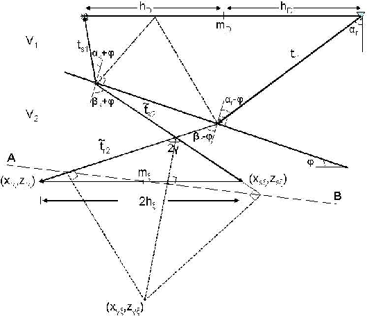
respectively. As illustrated in the sketch of
Figure 2, at any given depth the spatial coordinates of the
downward-continued source and receiver rays are given by:
are the half subsurface-offset and the depth of the image,
respectively. As illustrated in the sketch of
Figure 2, at any given depth the spatial coordinates of the
downward-continued source and receiver rays are given by:
where  is the water velocity,
  with
with  the sediment
velocity,
the sediment
velocity,  ,
,  are the takeoff angles of the source
and receiver rays with respect to the vertical and
are the takeoff angles of the source
and receiver rays with respect to the vertical and  and
and  are
the angles of the refracted source and receiver rays, respectively.
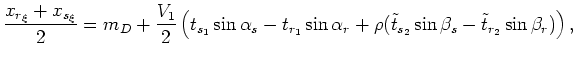
The coordinates of the migrated multiple in the image space are given by:
are
the angles of the refracted source and receiver rays, respectively.
The coordinates of the migrated multiple in the image space are given by:
The traveltime of the refracted ray segments
 and
and
 can be computed from the two imaging conditions: (1) at the image point the depth
of both rays has to be the same (since we are computing horizontal subsurface
offset gathers) and (2)
can be computed from the two imaging conditions: (1) at the image point the depth
of both rays has to be the same (since we are computing horizontal subsurface
offset gathers) and (2)
 which follows immediately
from equation 1 since at the image point the total extrapolated time
equals the traveltime of the multiple. As shown in Appendix A, the
traveltimes of the refracted rays are given by
which follows immediately
from equation 1 since at the image point the total extrapolated time
equals the traveltime of the multiple. As shown in Appendix A, the
traveltimes of the refracted rays are given by
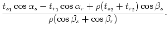
The refracted angles are related to the takeoff angles by Snell's law:
 and
and
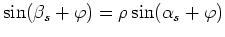 , from which we get
|
|---|
mul-sktch3
Figure 2. Imaging of water-bottom multiple
in SODCIG and ADCIG. The subscript  refers to the data space while the subscript refers to the data space while the subscript  refers to the image space.
The points refers to the image space.
The points
 and and
 represent the end points of the source
and receiver ray after migration and must be at the same depth at the image point (for horizontal ADCIGs).
The coordinates represent the end points of the source
and receiver ray after migration and must be at the same depth at the image point (for horizontal ADCIGs).
The coordinates
 correspond to the image point in the angle domain. The coordinates correspond to the image point in the angle domain. The coordinates
 correspond to the image point in the subsurface offset gather. The line AB represents
the apparent reflector at the image point. correspond to the image point in the subsurface offset gather. The line AB represents
the apparent reflector at the image point.
|
|---|
|
|
|---|
In ADCIGs, the mapping of the multiples can be directly related to the
previous equations by the geometry shown in Figure 2.
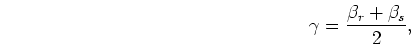
The half-aperture angle is given by
 |
(13) |
which is the same equation derived for converted waves by
(). The depth of the image point in ADCIGs
(
 ) is given by (Appendix B)
 |
(14) |
Equations 4-6 describe the
transformation performed by wave-equation migration between CMP gathers  and SODCIGs
. Equations 7-12 relate
the traveltimes and angles of the refracted segments to parameters that can in principle
be computed from the data (traveltimes, takeoff angles, reflector dips and velocities).
Equations 13 and 14 provide the transformation from
SODCIGs to ADCIGs.
These equations are valid for any
first-order water-bottom multiple, whether from
a flat or dipping water-bottom. They even describe the migration of
source- or receiver-side diffracted multiples with the diffractor at the
water bottom, since no assumption has been
made relating and or the individual traveltime segments.
These equations, however, are of little practical use unless
we can relate the individual traveltime segments (
and SODCIGs
. Equations 7-12 relate
the traveltimes and angles of the refracted segments to parameters that can in principle
be computed from the data (traveltimes, takeoff angles, reflector dips and velocities).
Equations 13 and 14 provide the transformation from
SODCIGs to ADCIGs.
These equations are valid for any
first-order water-bottom multiple, whether from
a flat or dipping water-bottom. They even describe the migration of
source- or receiver-side diffracted multiples with the diffractor at the
water bottom, since no assumption has been
made relating and or the individual traveltime segments.
These equations, however, are of little practical use unless
we can relate the individual traveltime segments ( ,
,  ,
,
 ,
,  ), and the angles and
to the known data space coordinates (, ,
), and the angles and
to the known data space coordinates (, ,  ) and the model parameters
(,
) and the model parameters
(,  and
and  ). This may not be easy or
even possible analytically for all situations, but it is for the simple
but important case of a specular multiple from a flat water-bottom.
). This may not be easy or
even possible analytically for all situations, but it is for the simple
but important case of a specular multiple from a flat water-bottom.
Next: Specular multiple from flat
Up: Kinematics of 2D multiples
Previous: Kinematics of 2D multiples
2007-10-24