Multiple Attenuation Results

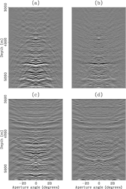
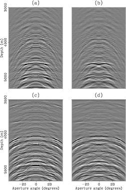
Rather than suppressing the multiples in the model domain, I chose to suppress the primaries and inverse transform the multiples to ADCIGs. This is more convenient because the primaries are not ``filtered'' through the imperfect forward-inverse Radon transform pair. The primaries were then recovered by directly subtracting the multiples from the data. I did not apply adaptive subtraction to obtain the results presented in this chapter. This is such an important issue that I designed a new algorithm for it and will present it in the next chapter. Figure 18 shows a close-up comparison of the primaries extracted with the standard 2D Radon transform (Sava and Guitton, 2003) and with the apex-shifted Radon transform for the two ADCIGs at the top in Figure 15. The standard transform (Figures 18a and 18c) was effective in attenuating the specular multiples, but failed at attenuating the diffracted multiples (below 4000 m), which are left as residual multiple energy in the primary data. Again, this is a consequence of the apex shift of these multiples. There appears not to be any subsalt primary reflections in Figures 18a and 18(b). The flattish reflector at about 4600 m in panel (b) is actually residual multiple energy (compare with panel (a)). Similarly for Figures 18(c) and 18(d). Figure 19 shows a similar comparison for the extracted multiples. Notice how the diffracted multiples were correctly identified and extracted by the apex-shifted Radon transform, in Figures 19(b) and  19(d). In contrast, the standard 2D transform misrepresent the diffracted multiples as though they are specular multiples as seen in Figures 19(a) and 19(c).

comp-prim1
Figure 18. Comparison of primaries extracted with the 2D Radon transform (a) and (c) and with the apex-shifted Radon transform (b) and (d). Notice that some of the diffracted multiples remain in the result with the 2D transform.

comp-mult1
Figure 19. Comparison of multiples extracted with the 2D Radon transform (a) and (c) and with the apex-shifted Radon transform (b) and (d).

In order to assess the effect of the improved attenuation of the diffracted multiples on the angle stack, I processed all ADCIGs. Figure 20 shows a close-up view of the stack of the primaries extracted with the standard Radon transform (panel (a)), the stack of the primaries extracted with the apex-shifted Radon transform (panel (b)), and their difference (panel (c)). All panels are plotted with the same plotting parameters. Notice that the diffracted multiple energy below the edge of the salt (5000 m to 7000 m) that appears as steeply-dipping noise with the standard transform, has been somewhat better attenuated with the apex-shifted transform. This is shown in detail in the difference panel in Figure 20(c). It is very difficult to identify any primary reflections below the edge of the salt, so it is hard to assess if the primaries have been equally preserved with both transforms. It is known, however, that for this dataset, there are no multiples above a depth of about 3600 m, between CMP positions 3000 m to 5000 m. The fact that the difference panel appears nearly white in that zone shows that the attenuation of the diffracted multiples did not affect the primaries. Of course, this is only true for those primaries that were correctly imaged, so that their moveout in the ADCIGs was nearly flat. Weak subsalt primaries may not have been well-imaged due to inaccuracies in the migration velocity field and 3D effects. These primaries, therefore, may have been attenuated with both the standard and the apex-shifted Radon transforms.

comp-prim1-stack
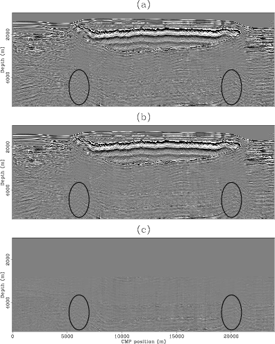
Figure 20. Comparison of angle stacks for primaries. Panel (a) corresponds to the primaries obtained with the standard Radon transform. Panel (b) corresponds to the primaries obtained with the apex-shifted Radon transform and panel (c) is the difference between panels (a) and (b). The ovals correspond to the diffracted multiples.

For the sake of completeness, Figure 21 shows the extracted multiples with the standard and the apex-shifted Radon transforms. Again, the main difference is largely in the diffracted multiples.

comp-mult1-stack
Figure 21. Comparison of angle stacks for multiples. Panel (a) corresponds to the multiple model computed with the standard Radon transform. Panel (b) corresponds to the multiple model computed with the apex-shifted Radon transform. Notice the difference in the attenuation of the diffracted multiples. The ovals correspond to the diffracted multiples.