Plane-wave source migration

Shot gathers can also be synthesized to a new dataset to represent a physical experiment that does not occur in reality. One of the most important examples is to synthesize shot gathers to plane-wave source gathers. The plane-wave source gathers represent experiments that planar sources originate from all angles at the surface. They can also be regarded as the accurate phase-encoding of the shot gathers Liu et al. (2006). The plane-wave source dataset can be generated by delaying the shot in shot gathers or slant-stacking in receiver gathers as follows:

$$R_p(p_x,p_y;r_x,r_y,z=0,\omega)=\int \int R(s_x,s_y;r_x,r_y,z=0,\omega)e^{i\omega (s_xp_x+s_yp_y)}ds_xds_y,$$ (4)

where p_x and p_y are ray parameters in the in-line and cross-line directions respectively. Its corresponding plane-wave source wavefield at the surface is

$$S_p(p_x,p_y;r_x,r_y,z=0,\omega)=\int\int e^{i\omega(s_xp_x+s_yp_y)}ds_xds_y.$$ (5)

Similar to the Fourier transformation, we can transform the plane-wave source data back to shot gathers by the inverse slant-stacking Claerbout (1985) as follows

$$R(s_x,s_y;r_x,r_y,z=0,\omega)= \int \int \omega^2 R_p(p_x,p_y;r_x,r_y,z=0,\omega)e^{-i\omega (s_xp_x+s_yp_y)} dp_xdp_y$$ (6)

In contrast to the inverse Fourier transformation, the kernel of the integral is weighted by the square of the frequency $\omega$.

The source wavefield S_p and receiver wavefield R_p are extrapolated into the subsurface independently using the one-way wave equations 1 and 2. The image of a plane-wave source with a ray parameter pair (p_x,p_y) is formed by cross-correlating the source and receiver wavefields weighted with the square of the frequency $\omega$:

$$I_{p_x,p_y}(x,y,z)=\int \omega^2 \bar{S_p}(p_x,p_y;x,y,z,\omega)R_p(p_x,p_y;x,y,z,\omega) d\omega.$$ (7)

The final image is generated by stacking the images of all possible plane-wave sources:

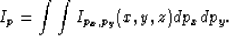$$I_{p}=\int\int I_{p_x,p_y}(x,y,z) dp_xdp_y.$$ (8)

Because both slant-stacking and migration are linear operators, the image of the plane-wave migration I_p is equivalent to the image obtained by shot-profile migration Liu et al. (2002); Zhang et al. (2005).