|
space
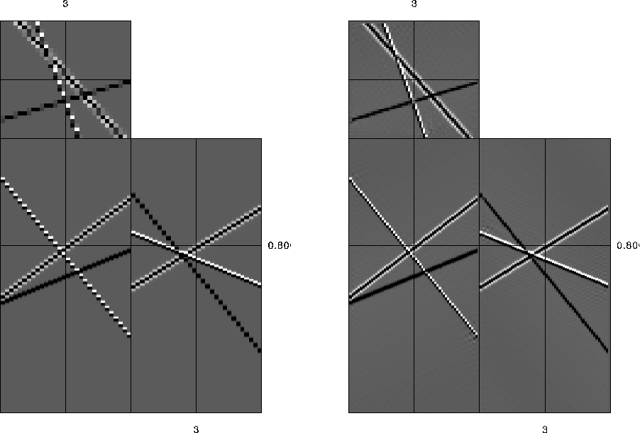
Figure 1 Left: PEF on output data; right: PEF spaced by a factor of two on input data with half the sampling in space. |  |
![[*]](http://sepwww.stanford.edu/latex2html/cross_ref_motif.gif) .
The amount of spacing corresponds to the factor of interpolation.
Once the PEF has been estimated on the input data, it is returned to the
original spacing and then the second step of the interpolation takes place,
where the interpolated model space is regularized by the PEF. This PEF is
estimated on the entire input dataset and is applied on the entire output dataset as
two global problems.
.
The amount of spacing corresponds to the factor of interpolation.
Once the PEF has been estimated on the input data, it is returned to the
original spacing and then the second step of the interpolation takes place,
where the interpolated model space is regularized by the PEF. This PEF is
estimated on the entire input dataset and is applied on the entire output dataset as
two global problems.
|
space
Figure 1 Left: PEF on output data; right: PEF spaced by a factor of two on input data with half the sampling in space. |  |
Interpolation in the f-x domain is performed by estimating a PEF for a single frequency; for a two-dimensional f-x scenario this would be a one-dimensional PEF along x. A unique PEF is estimated at each frequency of the input data, and this PEF is then used to regularize the output data at a higher frequency equal to the original frequency multiplied by the interpolation factor. In practice, the data used to create the PEF is padded in time before being transformed to frequency so that the frequencies after multiplication by the scale factor correspond to the output frequencies that are desired.
Because the f-x domain approach interpolates each frequency independently, the
input data can be broken along the frequency axis and interpolated in parallel or
sequentially. This means that the memory footprint of the f-x method is smaller
by a factor corresponding to the size of the time (or frequency) axis. Since
this is typically the largest axis, this can mean a reduction in the memory use
by two to three orders of magnitude. This savings of memory means that more
input data can be held in memory, and simultaneous interpolation of more
dimensions is possible with the f-x approach. For example, Figure ![[*]](http://sepwww.stanford.edu/latex2html/cross_ref_motif.gif) was quickly created on a laptop in a few minutes, whereas the same interpolation
in t-x would strain a larger workstation.
was quickly created on a laptop in a few minutes, whereas the same interpolation
in t-x would strain a larger workstation.
 |
The result shown in Figure ![[*]](http://sepwww.stanford.edu/latex2html/cross_ref_motif.gif) is interpolated by a factor of two
on three of the four axes. This type of approach not only provides a better
prediction by increasing the amount of input information but also speeds up the
interpolation process by simultaneously interpolating more dimensions, which
would require a cascade of lower-dimension interpolations with a t-x approach.
is interpolated by a factor of two
on three of the four axes. This type of approach not only provides a better
prediction by increasing the amount of input information but also speeds up the
interpolation process by simultaneously interpolating more dimensions, which
would require a cascade of lower-dimension interpolations with a t-x approach.
One reason why this f-x interpolation is much faster than t-x interpolation is that the t-x approach captures spectral information from the data which is not used during the interpolation. F-x PEFs are a much more compact and efficient way to capture the dip information in the training data. Also, the parameterization on the PEF in t-x is less intuitive than in f-x. In f-x, the size of the PEF roughly corresponds to the number of dips that it would be able to predict. In the t-x case, the length of the PEF in time also comes in to play as it relates to the maximum dip that could be predicted by the filter. Also, the spacing of the PEF assumes that the data are very oversampled in time, so if the data are not high-cut filtered before the PEF estimation the filter could be time-aliased. Since in f-x PEFs the lower frequencies are explicitly used to interpolate the higher frequencies this problem does not happen, although it also relies upon oversampling in time.