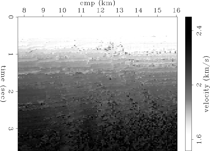
![[*]](http://sepwww.stanford.edu/latex2html/cross_ref_motif.gif) shows the RMS velocity.
shows the RMS velocity.
Real data from the Gulf on Mexico will now be examined. Figure
![[*]](http://sepwww.stanford.edu/latex2html/cross_ref_motif.gif) shows the RMS velocity.
shows the RMS velocity.
 |
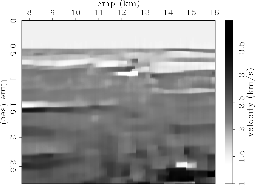
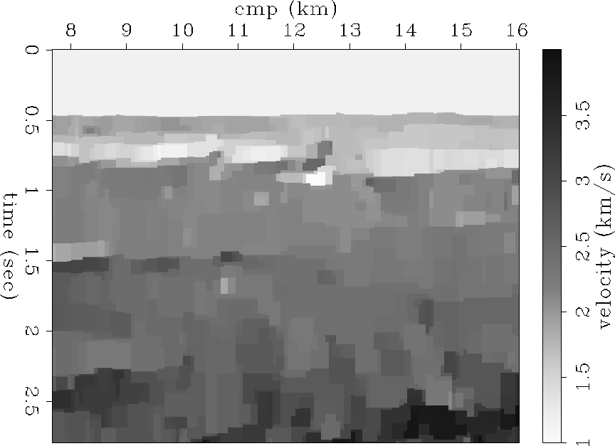
Figures ![[*]](http://sepwww.stanford.edu/latex2html/cross_ref_motif.gif) and
and ![[*]](http://sepwww.stanford.edu/latex2html/cross_ref_motif.gif) show the previous
inversion results done by Valenciano et al. (2003) and
Witten and Grant (2006), respectively. Notice that Figure
show the previous
inversion results done by Valenciano et al. (2003) and
Witten and Grant (2006), respectively. Notice that Figure
![[*]](http://sepwww.stanford.edu/latex2html/cross_ref_motif.gif) is smoother than Figure
is smoother than Figure ![[*]](http://sepwww.stanford.edu/latex2html/cross_ref_motif.gif) . This
is because Figure
. This
is because Figure ![[*]](http://sepwww.stanford.edu/latex2html/cross_ref_motif.gif) uses an approximate
uses an approximate ![]() norm.
norm.
 |
 |
The results from both previous inversion schemes have
limitations. Valenciano et al. (2003) uses an
approximate ![]() norm and has no stopping criterion. Thus it
requires as many iterations as the user is willing to execute. For the result
shown here, 800 conjugate gradient steps were taken. Witten and Grant (2006) is hampered by the use of the MATLAB based
icvx software Grant et al. (2006), limiting its use to small problems.
norm and has no stopping criterion. Thus it
requires as many iterations as the user is willing to execute. For the result
shown here, 800 conjugate gradient steps were taken. Witten and Grant (2006) is hampered by the use of the MATLAB based
icvx software Grant et al. (2006), limiting its use to small problems.
 |
![[*]](http://sepwww.stanford.edu/latex2html/cross_ref_motif.gif) and
and
![[*]](http://sepwww.stanford.edu/latex2html/cross_ref_motif.gif) . The smoothing along the midpoint axis does
not work.
. The smoothing along the midpoint axis does
not work.
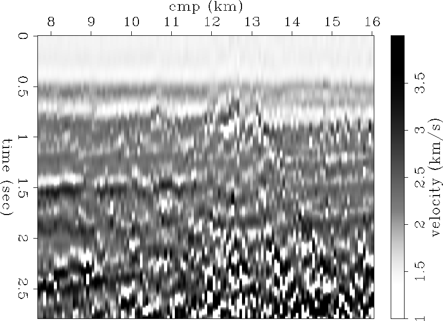
Although Figure ![[*]](http://sepwww.stanford.edu/latex2html/cross_ref_motif.gif) is not
perfect, the inversion result for the method
presented in this paper is close to the previous results. The
result in Figure
is not
perfect, the inversion result for the method
presented in this paper is close to the previous results. The
result in Figure ![[*]](http://sepwww.stanford.edu/latex2html/cross_ref_motif.gif) took only 108 iterations. All of the
major features are present in all three inversion results. The main
difference is in the smoothness of the result.
took only 108 iterations. All of the
major features are present in all three inversion results. The main
difference is in the smoothness of the result.