Downward-continuation migration

Claerbout (1999) introduces this concept and provides all the basic details for downward-continuation methods, including the survey-sinking concept. The explanation of all of these details is beyond the scope of this dissertation. I present only the basic concepts and describe how they can be adapted to converted-wave data.

The concept of survey-sinking is basically a downward continuation of the sources and the receivers. The shots and receivers can be downward continued to different depths during the process; however, they need to be at the same depth for the final image to be correct. To apply survey-sinking to converted-wave data the downward continuation of the source wavefield is carried out with the P-waves velocity, and the receiver wavefield is downward-continued with the velocity for the S-wave.

Using the concept of survey-sinking the final prestack $I(m_{\xi},z_{\xi})$ is obtained by taking the wavefield U at time equal zero (t=0),

$$I(m_{\xi},z_{\xi}) = U (s=m_{\xi},g=m_{\xi},z_{\xi},t=0).$$ (27)

where s, g, z represent the source position, the receiver position, and the reflector depth, respectively. For the final image to be correct, the data should migrate both to zero traveltime zero subsurface offset. This point in the image space also represents the conversion point for PS data. This is achieved with the correct velocity model. For the converted-wave case there will be two different velocity models.

The sinking or downward continuation of the wavefield at the surface (z=0) to a different depth level is described by  

$$U_{z} (\omega,m_\xi,h_\xi) = U_{z=0}(\omega,m_\xi,h_\xi) e^{iz {k_{z_{\bf s}}}} e^{iz {k_{z_{\bf g}}}}$$ (28)

This process is enabled by applying the Double Square Root (DSR) equation. In 2D this is described as follows

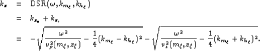$$\begin{eqnarray} k_z &=& {\rm DSR}(\omega,k_{m_\xi},k_{h_\xi}) \nonumber\ &=& ... ... \sqrt{\frac{\omega^2}{\vs2}-\frac{1}{4}(k_{m_\xi}+ k_{h_\xi})^2}.\end{eqnarray}$$ (29)

The final prestack image is extracted by summing all the frequencies at each depth level.

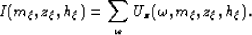$$I(m_\xi,z_{\xi},h_\xi) = \sum_{\omega} U_{z} (\omega,m_\xi,z_{\xi},h_\xi).$$ (30)

Different downward-continuation migration algorithms differ in the implementation of the DSR equation. This does not impact the results presented in the following sections. As mentioned before, in both the P-waves and the S-waves velocities, the energy should collapse to zero subsurface-offset. However, we can extract more information from our image - that is velocity information - by transforming the subsurface offset into angle information. Chapter 3 describes this process for converted-wave data and presents both a synthetic and a real data examples.