


Zhou et al. (1996) discuss that Hale's 1984 DMO operator via a Fourier transform is computationally expensive because the DMO operator is temporally nonstationary. They use the technique of logarithmic time stretching, first introduced by Bolondi et al. (1982) to present another derivation for the frequency-wavenumber log-stretch DMO operator.
Xu et al. (2001) exploit the idea of computational efficiency of the logarithmic time stretching for the PS-DMO operator. I reformulate the work of Xu et al. (2001) using the PS-DMO smile derived in the previous section and following a procedure similar to Hale (1984) and Zhou et al. (1996). This operation is valid for a constant velocity case.
From equation ![[*]](http://sepwww.stanford.edu/latex2html/cross_ref_motif.gif) , and following
Hale's 1984 assumption that
the DMO operator maps each sample of the NMO section (pn)
from time tn to time t0 without changing its
midpoint location, x [p0(t0,x,h) = pn(tn,x,h)],
the 2-D PS-DMO operator in the f-k domain is
, and following
Hale's 1984 assumption that
the DMO operator maps each sample of the NMO section (pn)
from time tn to time t0 without changing its
midpoint location, x [p0(t0,x,h) = pn(tn,x,h)],
the 2-D PS-DMO operator in the f-k domain is
| |
(16) |
Equation () implies a change of variable from t0 to tn.
From equation () we have
| (17) |
| (18) |
which I will represent as A or its Fourier equivalent:
| (19) |
becomes
| |
(20) |
Equation () is the foundation of PS-DMO in the f-k domain.
I introduce a time log-stretch transform pair,
 |
(21) | |
| (22) |
where tc is the minimum cutoff time introduced to avoid taking the logarithm of zero. The PS-DMO operator in the f-k log-stretch domain becomes
| |
(23) |
where
| (24) |
with
 |
(25) |
where ![]() is the Fourier representation of the log-stretched time axis
is the Fourier representation of the log-stretched time axis ![]() . The value
of the function
. The value
of the function ![]() for either kh =0 or
for either kh =0 or ![]() is obtained as zero by
taking the limit of the function
is obtained as zero by
taking the limit of the function ![]() for either
for either ![]() or
or ![]() and applying the L'Hopital's rule.
and applying the L'Hopital's rule.
The previous expression is equivalent to the one presented by Xu et al. (2001).
Note that
equation () is based on the assumption that p0(t0,x,h) =
pn(tn,x,h).
This does not include changes in midpoint position and/or common reflection
point position.
This leads to a correct kinematic operator but one with a poor amplitude
distribution along steeply dipping
reflectors.
Zhou et al. (1996) solve this problem for PP-DMO in the f-k log-stretch
domain by reformulating the f-k log-stretch PP-DMO operator
presented by Black et al. (1993). This
operator is based on the
assumption that the midpoint changes its location after the
PP-DMO operator is applied [p0(t0,x0,h) = pn(tn,xn,h)], which leads
to a more accurate distribution of amplitudes.
Following the derivation used by Zhou et al. (1996) for PP-DMO, for steeply dipping
events I derive a more accurate
PS-DMO operator in the frequency-wavenumber log-stretch domain.
This new operator differs from the previous one in the function
![]() of the filter
of the filter ![]() . The new expression is
. The new expression is
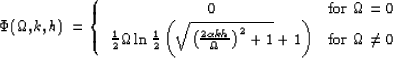
![\begin{displaymath}
\Phi(\Omega,k,h) = \left \{ \begin{array}
{cc}
\alpha kh & ...
... ]} \right \} & \mbox{for $\Omega \ne 0$}
\end{array} \right .\end{displaymath}](img43.gif) |
(26) |
The values of the phase-like function ![]() at the points kh =0 and
at the points kh =0 and ![]() are obtained using L'Hopital's rule on the limit of the function
are obtained using L'Hopital's rule on the limit of the function ![]() , since
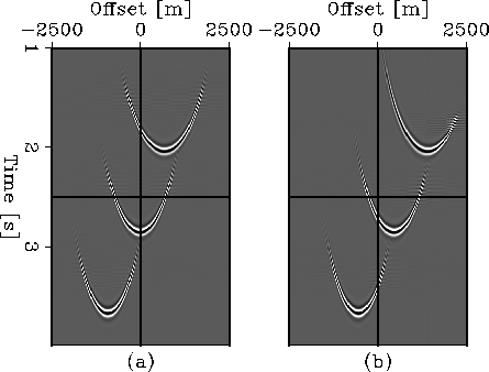
the function is singular at those points. Figure shows a series of impulse responses for this
operator.
, since
the function is singular at those points. Figure shows a series of impulse responses for this
operator.
 |
![[*]](http://sepwww.stanford.edu/latex2html/movie.gif)


Note that for a value of ![]() , equivalent to
, equivalent to ![]() , the
filter reduces to the known expression for P-wave data Zhou et al. (1996).
We can trust the PS results since
the PP impulse response, obtained with the filter in
equation and
, the
filter reduces to the known expression for P-wave data Zhou et al. (1996).
We can trust the PS results since
the PP impulse response, obtained with the filter in
equation and ![]() , is
the same as that obtained by Zhou et al. (1996). Moreover, the amplitude distribution follows
Jaramillo's 1997 result.
The 3-D representation for this PS-DMO operator is the
starting point for the partial-prestack migration operator presented in
Chapter 4.
, is
the same as that obtained by Zhou et al. (1996). Moreover, the amplitude distribution follows
Jaramillo's 1997 result.
The 3-D representation for this PS-DMO operator is the
starting point for the partial-prestack migration operator presented in
Chapter 4.