

Next: 3D results from Gulf
Up: 2D Test Cases
Previous: Missing Chunks of data
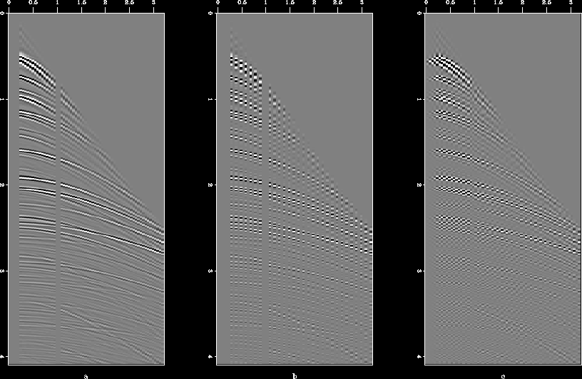
The most challenging part of the interpolation problem is to go beyond aliasing. This proves to be the acid test for various interpolation schemes. The method proposed in this paper has difficulties going beyond aliasing, as is illustrated with the help of a few examples. Figure ![[*]](http://sepwww.stanford.edu/latex2html/cross_ref_motif.gif) (a) shows a synthetic data set (called "hask", a CMP gather with a hole) which I will use to test the method. Figure
(a) shows a synthetic data set (called "hask", a CMP gather with a hole) which I will use to test the method. Figure ![[*]](http://sepwww.stanford.edu/latex2html/cross_ref_motif.gif) (b) shows the missing data set created from the original by throwing away every alternate trace, and the result of interpolation is given in Figure
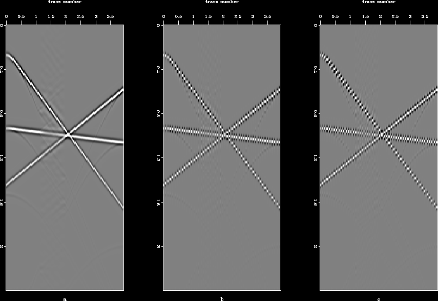
(b) shows the missing data set created from the original by throwing away every alternate trace, and the result of interpolation is given in Figure ![[*]](http://sepwww.stanford.edu/latex2html/cross_ref_motif.gif) (c). As can be seen, results are poor, the covariance-based filter catches the aliased trends. Another example for which the method fails is that of three plane waves. Figure
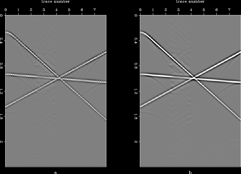
(c). As can be seen, results are poor, the covariance-based filter catches the aliased trends. Another example for which the method fails is that of three plane waves. Figure ![[*]](http://sepwww.stanford.edu/latex2html/cross_ref_motif.gif) shows the original data set, the data set with missing traces, and the interpolated result. In this case too, we end up estimating the covariance and filter based on the aliased trends. Stationary 2D PEFs (different shapes and sizes) also failed to interpolate satisfactorily for the synthetic data set, results for a 10
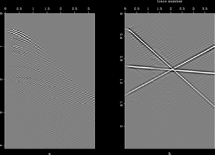
shows the original data set, the data set with missing traces, and the interpolated result. In this case too, we end up estimating the covariance and filter based on the aliased trends. Stationary 2D PEFs (different shapes and sizes) also failed to interpolate satisfactorily for the synthetic data set, results for a 10 5 PEF with 1000 iterations are given in Figure
 ![[*]](http://sepwww.stanford.edu/latex2html/cross_ref_motif.gif) (a). PEFs performed well on the example of three plane waves, as demonstrated in Figure
(a). PEFs performed well on the example of three plane waves, as demonstrated in Figure ![[*]](http://sepwww.stanford.edu/latex2html/cross_ref_motif.gif) (b).
(b).
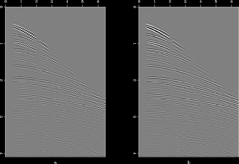
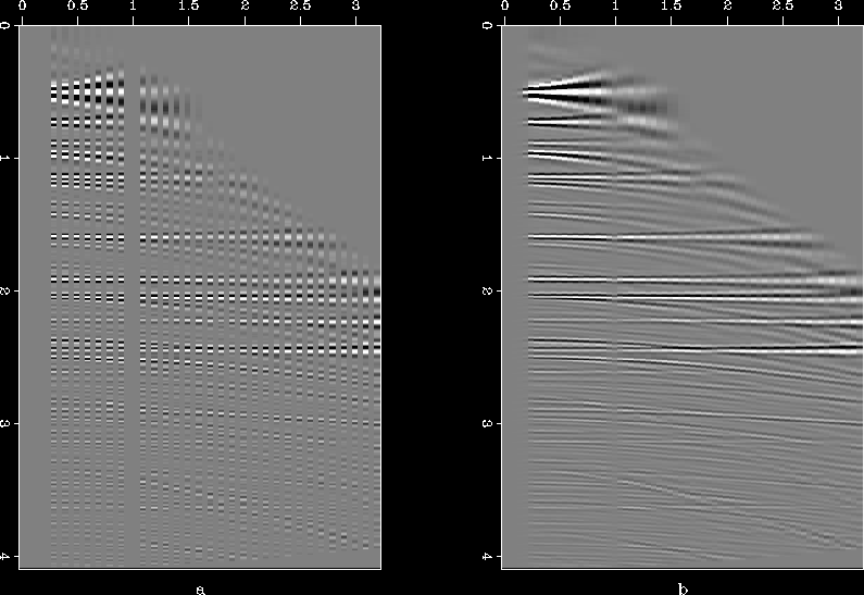
The results presented above might suggest that the method cannot handle crossing or multiple dips. This would definitely be unfortunate, especially in the context of seismic data which need not have regular, pre-defined patterns. I show with the help of a few examples that it is the aliasing and not the presence of multiple dips that is the source of problem. Figure ![[*]](http://sepwww.stanford.edu/latex2html/cross_ref_motif.gif) (a) is the same synthetic data set that was used above, with zero traces inserted in between; as a result the data is not aliased but has multiple and conflicting dips. Figure
(a) is the same synthetic data set that was used above, with zero traces inserted in between; as a result the data is not aliased but has multiple and conflicting dips. Figure ![[*]](http://sepwww.stanford.edu/latex2html/cross_ref_motif.gif) (b) is the interpolated result. Results of a similar exercise for the plane-wave example are given in Figure
(b) is the interpolated result. Results of a similar exercise for the plane-wave example are given in Figure ![[*]](http://sepwww.stanford.edu/latex2html/cross_ref_motif.gif) .
.
haskf
Figure 9 (a) Synthetic data set (called "hask"), (b) alternate missing traces, and (c) result after interpolation.
stlinesf
Figure 10 (a) Three plane waves, (b) alternate traces missing, and (c) result after interpolation.
compef
Figure 11 Results obtained with PEF for (a) hask and (b) plane waves.
hasks
Figure 12 (a) Synthetic data set with zero traces inserted in between, and (b) reconstructed result.
stliness
Figure 13 (a) Three plane waves with zero traces inserted in between, and (b) reconstructed result.
Aliasing is related to both the steepness of dips and the sampling rate. One way to get around this problem, at least with CMP gathers, is to apply interpolation after flattening using NMO Ji and Claerbout (1991). In an ideal case when velocity information is perfect, gathers are absolutely flat, but even if they are not, anything approaching flat gathers is good enough for interpolation. In the limiting case where everything is perfectly flat, linear interpolation will do as well as any other method. Figure ![[*]](http://sepwww.stanford.edu/latex2html/cross_ref_motif.gif) (a) shows NMOed missing data corresponding to Figure
(a) shows NMOed missing data corresponding to Figure ![[*]](http://sepwww.stanford.edu/latex2html/cross_ref_motif.gif) (b), and figure
(b), and figure ![[*]](http://sepwww.stanford.edu/latex2html/cross_ref_motif.gif) (b) shows the result of interpolation.
(b) shows the result of interpolation.
nhask
Figure 14 (a) NMOed synthetic data set, with missing traces, and (b) reconstructed result.
When we address the problem of interpolation beyond aliasing, either we should introduce some kind of model styling to exploit the information we have about the model, or we should generate some kind of proxy data. In this article, I briefly discuss three such methods of generating the proxy data that have imperfect, but still promising results, and I present results for one of them. Using the techniques presented below, I create a proxy data onto which I estimate the covariance-based filter and then interpolate the original data.
- 1.
- The crudest way of making the covariance estimator pick the trends we want is to generate a proxy data by linear interpolation along the known dips. The method first estimates the dips on the aliased data, and then does linear interpolation along those dips. Once we have the results from linear interpolation, we can estimate our covariance-based interpolation filter on this data, and then repeat the process of interpolation with the estimated filter. The results obtained from this technique were good, but this method has a severe shortcoming: it restricts the solution to a finite number of choices in terms of dips, and in places with conflicting dips, this might enhance one dip relative to the other. On certain occasions, low-energy events might be of interest, and in the presence of high-energy events, the dip estimator might miss the low-energy events, eliminating them from the solution. As a result, in spite of promising first results I was discouraged from using this method.
- 2.
- A second, more sophisticated approach is to use the pyramid-domain representation of the aliased data Burt and Adelson (1983); Sen (2006). It is a low-frequency representation on higher-level pyramids and can potentially be useful for removing aliasing artifacts. Initial results with this method were not good, but with more work, this technique might be exploited to handle problems of aliasing.
- 3.
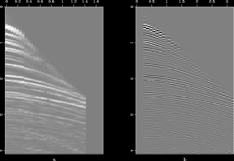
- The last approach presented here is that of creating envelopes to arrive at a low-frequency unaliased representation of the original data. The standard approach is to take the Hilbert transform, and then estimate the absolute value Claerbout (1992). Since that would be an extremely low-frequency representation, inadequate for estimation of covariances, I take the absolute value without taking the Hilbert transform. Strictly speaking, this is not the envelope, but an intermediate-frequency representation rather than a low-frequency one. Figure
![[*]](http://sepwww.stanford.edu/latex2html/cross_ref_motif.gif) (a) shows the envelope (absolute value), and Figure
(a) shows the envelope (absolute value), and Figure ![[*]](http://sepwww.stanford.edu/latex2html/cross_ref_motif.gif) (b) is interpolated result. As can be noticed, results are not perfect but much better than results shown in figure
(b) is interpolated result. As can be noticed, results are not perfect but much better than results shown in figure ![[*]](http://sepwww.stanford.edu/latex2html/cross_ref_motif.gif) (c)
(c)
haskt
Figure 15 (a)Psuedo-envelope for hask data, and (b) results obtained with envelopes.


Next: 3D results from Gulf
Up: 2D Test Cases
Previous: Missing Chunks of data
Stanford Exploration Project
1/16/2007
![[*]](http://sepwww.stanford.edu/latex2html/cross_ref_motif.gif) (a) is the same synthetic data set that was used above, with zero traces inserted in between; as a result the data is not aliased but has multiple and conflicting dips. Figure
(a) is the same synthetic data set that was used above, with zero traces inserted in between; as a result the data is not aliased but has multiple and conflicting dips. Figure ![[*]](http://sepwww.stanford.edu/latex2html/cross_ref_motif.gif) (b) is the interpolated result. Results of a similar exercise for the plane-wave example are given in Figure
(b) is the interpolated result. Results of a similar exercise for the plane-wave example are given in Figure ![[*]](http://sepwww.stanford.edu/latex2html/cross_ref_motif.gif) .
.
