Missing Chunks of data

In this section we look at some cases where instead of alternate missing traces we have big chunks of missing data. In the approach described above, the interpolation filter makes use of the four nearest diagonal neighbors to estimate the missing values, but in cases of big chunks of missing data, this approach can not be extended directly, due to lack of any diagonal neighbor in the middle of the hole. What we can do alternatively is to use nearest non-zero diagonal neighbors instead of nearest diagonal neighbors, maintaining the symmetry so that we maintain the same directional covariances. Equation 8 describes how we can use columns situated far apart for interpolation.  

$$P_{i,j} = \alpha_1 P_{i-h,j-h} + \alpha_2 P_{i+h,j-h} + \alpha_3 P_{i-h,j+h} + \alpha_4 P_{i+h,j+h} ,$$ (8)

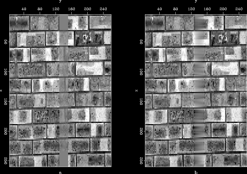
where h is the distance to nearest non-zero column. Figure (a) shows a texture made up of bricks, which again is more or less stationary, complying with the initial assumptions. If we create a hole of missing data as shown in Figure (b) and use a filter which instead of using nearest diagonal neighbors uses the tenth nearest diagonal neighbor (still a four point filter but ten times larger in size, as the coefficients are spaced ten points apart), we do a reasonable job of estimating the missing values as displayed in figure (a). Since the filter is much larger, it has pronounced boundary effects as can be noticed. Comparing the results obtained using this approach with those obtained with PEF (figure (b)), the main difference is that this approach maintains the same covariance within the missing chunk as measured from the data, whereas missing values obtained by PEF appear to be of lower frequency than actual values. 2D PEFs of size 5$\times$5 with 500 iterations were used for all the examples presented in this section. Incidentally, the brick example happens to be a case where everything required by the covariance-based interpolation algorithm falls in place and results are good, it does not work equally well for all the cases in general, as discussed with the help of later examples.

 

brickf1
Figure 4 (a)Texture made up of bricks, and (b) texture with a missing block of data.

 

brickf2
Figure 5 Reconstructed brick texture with (a) covariance-based approach, and (b) PEF.

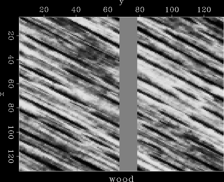
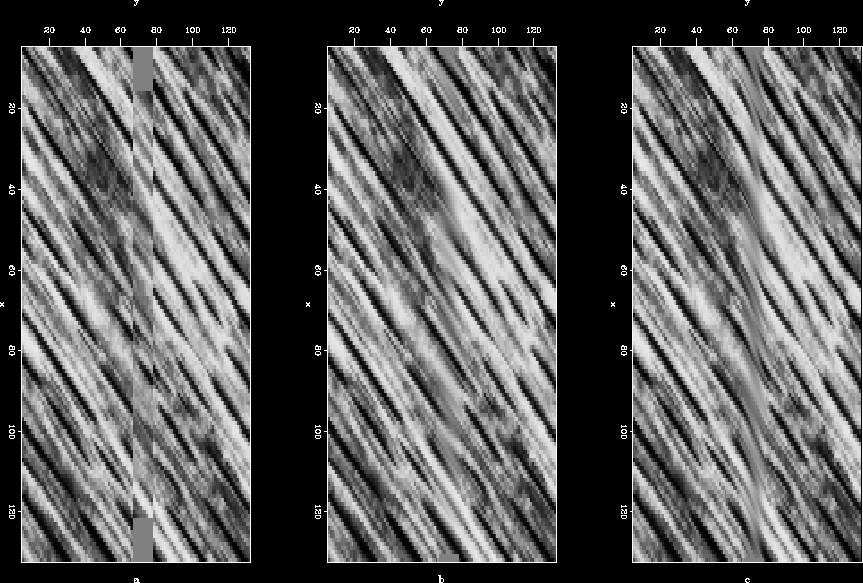
This approach of multi-scaling worked well for the brick example in spite of scaling the filter by a factor of 10 (incidentally), but it has a severe limitation. When we use values situated far apart from actual point of interest, we by no means ensure continuity at the edges of the hole. This is illustrated with the help of the previously used wood texture. Figure shows the missing data, and (a) is the image after interpolation. A sharp discontinuity is visible at the edges of the hole. In this case, the results of PEF are much better, as can be observed from Figure (b). PEF in this case performs better, primarily because it formulates the problem of filling the missing values as an inverse problem and introduces some kind of regularization. On the other hand in the covariance-based approach, estimation of missing values is just a one-step process, and no constraints can be levied. Only thing to appreciate about filling with the covariance-based approach is that it maintains the same texture in terms of frequency content.

 

woods1
Figure 6 Wood texture with missing hole of data.

 

woods2
Figure 7 Reconstructed wood texture interpolated with (a) current approach, (b) PEF, and (c) modified iterative approach.

There are different ways to attack the problem of bigger sized holes. One approach is to use an adaptable filter to interpolate, rather than a fixed large filter as was used above. In this case we do not ensure that filter is scaled equally in all directions; rather we let it expand independently in all directions until it hits a non-zero value, then freeze the size there and use that filter to interpolate. Results obtained using this method were not encouraging, possibly because we do not maintain symmetry in the filter. Symmetry should be maintained at all scales to preserve the directional covariance.

Another approach is to interpolate iteratively. Consider a situation where the hole is of size h and is located at the jth position from left. When we interpolate any pixel belonging to the jth column using an unscaled filter and its four diagonal neighbors, we encounter two missing values corresponding to column j+1, and two known values corresponding to column j-1. As a result of this interpolation, we get nonzero values in column j and in column j+h (which is at the other side of the hole). Although this value is a step in the right direction, it is far from the actual value. We can repeat this process until we completely fill the hole.

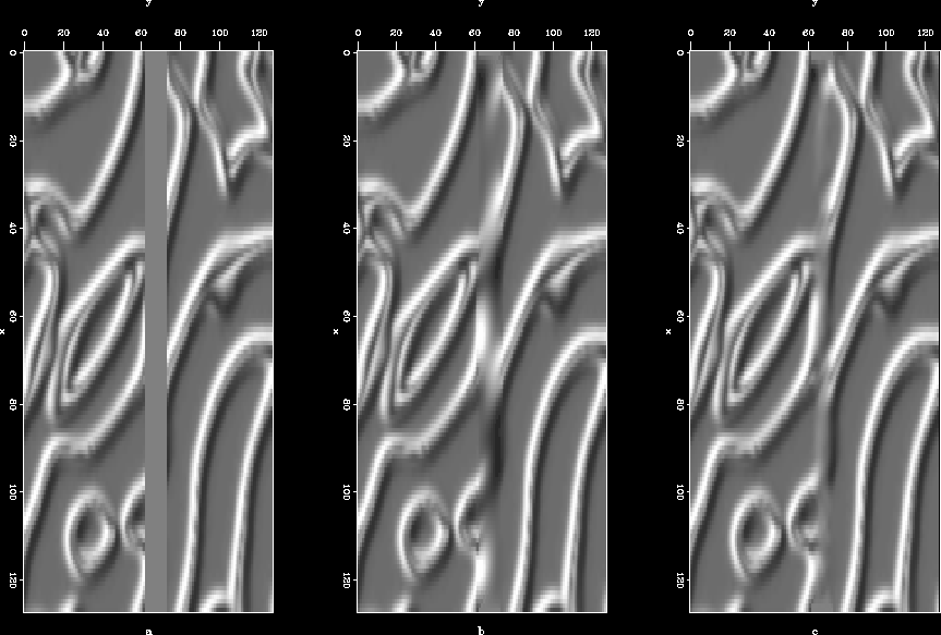
Results of the iterative scheme described above for the same wood texture are given in Figure (c). As can be seen, results are marginally better and maintain the image continuity, but they are still far from the true value. The results of the same experiment carried out on the ridges texture are given in Figure . Figure (a) shows the missing data, Figure (b) shows the result of interpolating with the iterative covariance-based scheme, and Figure (c) shows the result of interpolating with PEFs. On lower part of the hole iterative scheme proposed here seems to work a little better than PEFs in terms of getting the curvature and also, the amplitudes in middle of the hole look a little better in the results obtained by iterative covariance-based algorithm.

 

ridgess
Figure 8 (a) Missing data in ridges, reconstructed with (b) modified iterative scheme and (c) PEF.