Sigsbee 2b synthetic examples

The Sigsbee2B dataset was designed to model strong surface-related multiples from an offshore acquisition. Two datasets were generated with a 2D finite difference algorithm: One with the perfectly reflecting free surface, and one without. Therefore, the direct subtraction of the two data volumes yields a perfect multiple model (modulo source and receiver ghost effects), without the need for SRMP. Though the data were modeled with an off-end acquisition strategy, split-spread gathers were computed via reciprocity for all of the examples below.

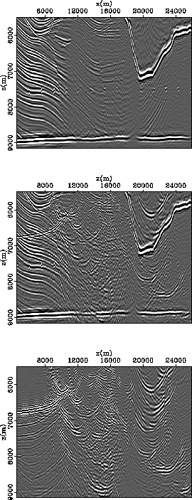
Figure 2 shows three versions of the bottom third of the image produced with the Sigsbee2b data sets. The top image used the data modeled without the reflecting free surface and contains only primaries. The middle image migrated the data with the free-surface and contains multiples as well. The bottom panel is the image produced by migrating the difference between the two data volumes (only multiples). The complex multiples in this deep section quickly overwhelm the primary events and could easily be mistaken for primaries in some instances. All panels, and the rest of the images herein, were produced with four reference velocities in a PSPI shot-profile migration code.

 

GEO-2006-0199-fig2
Figure 2 Images of the bottom third of Sigsbee2b modeled data. Top panel is migration of primaries only. Middle panel is migration of multiples and primaries. Bottom panel is migration of multiples only.

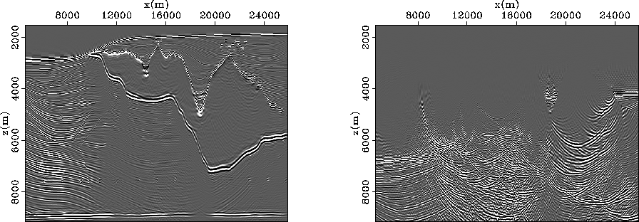
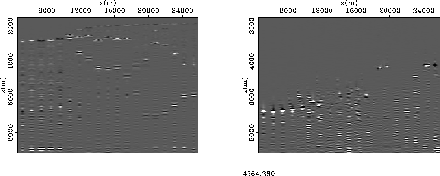
Figure 3a shows the zero subsurface-offset image from the data modeled without the free surface (multiple free). Panel b was produced with the same data and the IS-SRMP imaging condition, equation 8. By autoconvolving the upcoming wavefield U at every depth level in the image space, the right panel shows only multiples in the image domain using data containing only primaries. Note that there is no energy in Panel b above the first water-bottom multiple.

 

GEO-2006-0199-fig3
Figure 3 Zero subsurface-offset images of Sigsbee 2b data without the free surface. Panel a used conventional shot-profile imaging condition (equation 3). Panel b used the multiple prediction imaging condition for IS-SRMP. (equation 9).

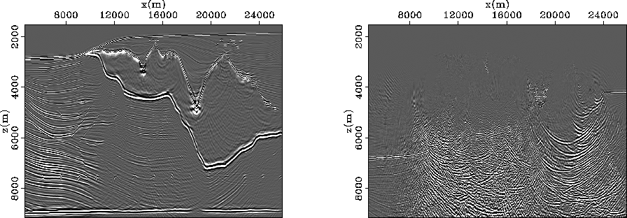
Figure 4 is directly analogous to the images in Figure 3, though employed the deconvolution imaging conditions from equations 16 & 17 respectively. Notice the increased bandwidth of the events in Panel b compared to the previous result and the increased quality of the steeply dipping salt bottom in Panel a. Also, in the shallow depths before the first water-bottom multiple and within the salt body, the multiple prediction shows increased noise/chatter. This can be muted before (adaptive) subtraction and should pose little problem.

 

GEO-2006-0199-fig4
Figure 4 Deconvolutional imaging conditions used in contrast to Figure 3. Panel a used shot-profile imaging condition with deconvolution (equation 16). Panel b used the multiple prediction imaging condition with deconvolution (equation 17).

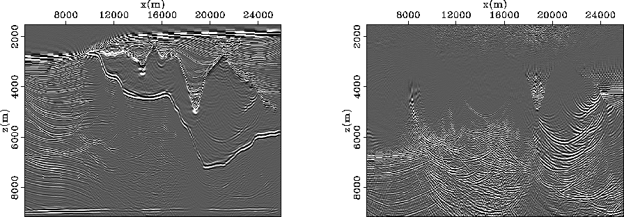
Figures 5 & 6 are images produced with conventional and deconvolutional imaging conditions, respectively, using the data containing primaries and multiples. The multiples below the salt body, which may be difficult to label as such without prior knowledge, are well predicted.

 

GEO-2006-0199-fig5
Figure 5 Zero subsurface-offset images of Sigsbee 2b data with the free surface. Panel a used conventional shot-profile imaging condition (equation 3). Panel b used the multiple prediction imaging condition (equation 9).

 

GEO-2006-0199-fig6
Figure 6 Deconvolutional imaging conditions used in contrast to Figure 5 (free surface included). Panel a used shot-profile imaging condition with deconvolution, (equation 16). Panel b used the multiple prediction imaging condition with deconvolution (equation 17).

Guitton (2005) shows convincingly that pattern-based and adaptive subtraction of multiple models work much better when higher dimensinalities can be exploited by the subtraction algorithm. The various imaging conditions presented above can all calculate subsurface offset dimensions to facilitate better subtraction. Figure 7 shows the extension of the imaging conditions above to non-zero reflection angle Sun et al. (2004). The data were migrated using the imaging conditions above, and then transformed to the angle domain after Sava and Fomel (2003). The data input to migration contained both primaries and multiples, and the imaging conditions used were not the deconvolutional variants.

 

GEO-2006-0199-fig7
Figure 7 Angle-domain common-image gathers selected regularly across the image. Panel a used the conventional imaging condition (equation 3), Panel b the multiple prediction imaging condition (equation 9). The volumes were then transformed to incidence/reflection angle.