Image-space SRMP

To predict multiples in the image space, the transform from the data space (shot gathers) to the image space plays an integral role. The image space is the output of migration, which in this implementation, is produced with a shot-profile depth migration algorithm. Shot-profile wave-equation depth migration Claerbout (1971) is the cascade of two component operations: extrapolation, and imaging. The extrapolation is carried out with an anticausal wave-equation operator on the up-going wavefield, U, and a causal operator for the down-going wavefield, D. U is a shot record with traces placed along a wavefield axis ${\bf x}$. D is a zero valued wavefield, also defined along the axis ${\bf x}$ where a source function is placed at the location of the shot being migrated, ${\bf x}_s$. The wavefields are recursively extrapolated to all depths z using the one-way Fourier domain solution to the wave-equation

$$\begin{eqnarray} U_{z+1}({\bf k}_x;{\bf x}_s,\omega)&=& U_{z}({\bf k}_x;{\bf ... ...& D_{z}({\bf k}_x;{\bf x}_s,\omega) \mbox{exp}(-i\omega k_z) \;. \end{eqnarray}$$ (1) (2)

In this work, the form of the dispersion relation used to calculate the vertical wavenumber, k_z, is the phase-shift plus interpolation (PSPI) algorithm Gazdag and Sguazzero (1984), though the degree of complexity of the operator does not change the discussion herein. The importance of these equations is that the operator that extrapolates a wavefield from one depth level to the next is a diagonal square matrix.

The correlation based multi-offset imaging condition for shot-profile migration at each depth level z is Rickett and Sava (2002)  

$$i_z({\bf x},{\bf h})= \sum_{{\bf x}_s}\sum_\omega U_z (... ...};{\bf x}_s,\omega) D_z^*({\bf x}-{\bf h};{\bf x}_s,\omega)\;$$ (3)

where the * represents conjugation. Extraction of the zero lag of the correlations, by summation over $\omega$, combines the energy in the two wavefields that is colocated at each depth level. Overlapping acquisition patches from the individual shots are stacked by the sum over ${\bf x}_s$.

SRME is also a two component process: Multiple prediction and subtraction. Acknowledging the approximation of autoconvolving raw data traces rather than convolving data with only primaries, the prediction step (SRMP) can be written in the Fourier domain (Berkhout and Verschuur, equation 13f, 1997)  

$$M({\bf x}_g;{\bf x}_s,\omega)=\sum_{{\bf x}_a} R({\bf x}_g;{\bf x}_a,\omega) R({\bf x}_a;{\bf x}_s,\omega)\;,$$ (4)

where R is the data-space volume of shot-gathers defined at geophone and source locations on the acquisition surface. Equation 4 is a trace-by-trace operation to produce the multiple prediction with any geophone-source, $({\bf x}_g,{\bf x}_s)$, combination by convolving each trace of every shot gather with all the others followed by summing over the convolution index ${\bf x}_a$. Note however, the similarity of the SRMP equation to the imaging condition of shot-profile migration, equation 3.

Wave-equation extrapolation is performed on wavefields where data and source-functions are used as initial conditions to propagate energy into the subsurface. To begin, traces at locations ${\bf x}_g$ are inserted into a zero-valued wavefield defined along the axis ${\bf x}$ as depicted in Figure 1. Although data-space SRMP is a trace-by-trace operation, equation 4 can be redefined in terms of the wavefield $U({\bf x},{\bf x}_s)$. Because null-traces occupy locations ${\bf x}$ at which no data were collected, a multiple prediction can be also be written  

$$M_{z=0}({\bf x};{\bf x}_s,\omega)=\sum_{{\bf x}_a} U_{z=... ...f x};{\bf x}_a,\omega) U_{z=0}({\bf x}_a;{\bf x}_s,\omega)\;,$$ (5)

where the resultant volume has been regularized along ${\bf x}$ by adding zero-traces, and we have added the specification that the operation is being performed at the recording surface z=0.

 

GEO-2006-0199-fig1 Figure 1 Traces from a shot-gather at locations 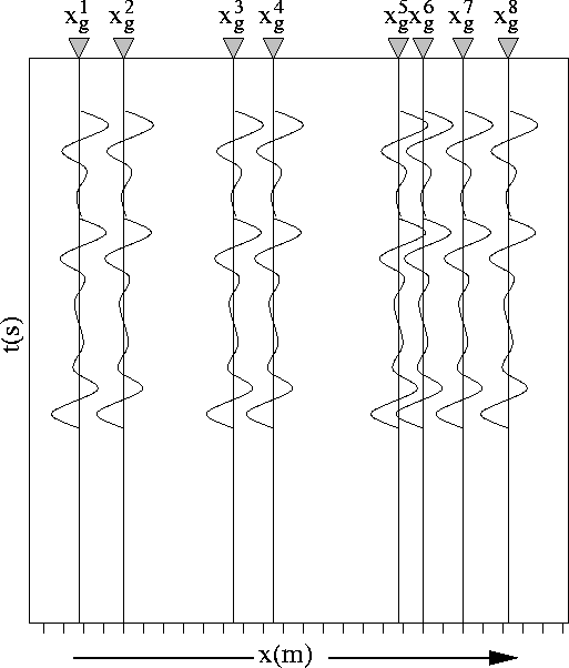${\bf x}_g^i$ are inserted along the ${\bf x}$ axis to define the initial conditions for the upcoming wavefield U.

Using the principle of reciprocity between the receiver and source locations (first and second arguments of the wavefields respectively), the multiple prediction becomes  

$$M_{z=0}({\bf x};{\bf x}_s,\omega)=\sum_{{\bf x}_a} U_{z=... ...f x};{\bf x}_a,\omega) U_{z=0}({\bf x}_s;{\bf x}_a,\omega)\;,$$ (6)

where the subscript s on the RHS now represents simply a different receiver location (since it is the first argument of the wavefield), and the dummy index ${\bf x}_a$ is recognized as a summation over source location. Therefore, using arbitrary index subscripts c,d and restoring the significance of source location to subscript s  

$$M_{z=0}({\bf x}_c;{\bf x}_d,\omega)=\sum_{{\bf x}_s} U_{... ...x}_c;{\bf x}_s,\omega) U_{z=0}({\bf x}_d;{\bf x}_s,\omega)\;.$$ (7)

Finally, we define the dummy indices c,d in terms of physically significant variables location and half-offset, ${\bf x}_c={\bf x}+{\bf h}$ and ${\bf x}_d={\bf x}-{\bf h}$, such that  

$$M_{z=0}({\bf x},{\bf h},\omega)= \sum_{{\bf x}_s} U_{z=... ...\bf x}_s,\omega) U_{z=0}({\bf x}-{\bf h};{\bf x}_s,\omega)\;.$$ (8)

Thus reconfigured, equation 8 is now of parallel construction to the shot-profile imaging condition, equation 3, lacking only the summation over frequency.

Extrapolation by the exponential phase-shift operator $\mbox{exp}(+i\omega k_z)$, in equation 1, simply redatums the shot-gather U. Image-space SRMP (IS-SRMP) is the application of a second imaging condition evaluated at each subsurface depth level during the migration that images only multiples. It is the chain of multiple prediction (convolution) and zero-time extraction (summation over frequency). The image-space multiple prediction, as a function of sub-surface offset, is therefore  

$$m_z({\bf x},{\bf h})= \sum_{{\bf x}_s}\sum_\omega U_z({... ...h};{\bf x}_s,\omega) U_z({\bf x}-{\bf h};{\bf x}_s,\omega)\;.$$ (9)

There are two important ramifications for the equation for predicting multiples with the imaging condition above. The first, is that this operation is intrinsically a shot-domain manipulation of the data. After sorting to CMP-offset coordinates, the source and receiver coordinates are mixed in such a way as to make IS-SRMP invalid for survey-sinking style migration algorithms. Second, because reciprocity was invoked to derive equation 9, off-end (marine) acquisition geometries will need to have split-spread gathers manufactured via reciprocity. The split-spread gathers will include the ray-paths from multiples that emerge in front of the receiver spread (boat) which need to be included in the shot-gathers to predict all possible multiple events.

Further understanding of the IS-SRMP imaging condition for those familiar with shot-profile migration algorithms can be elicited by defining the down-going wavefield in equations 1 & 2 by $D\equiv U$. Therefore, equations 1 - 3 become

$$\begin{eqnarray} U_{z+1}({\bf k}_x;{\bf x}_s,\omega)&=& U_{z}({\bf k}_x;{\bf ... ...\hat{U}_{z}({\bf k}_x;{\bf x}_s,\omega) \mbox{exp}(-i\omega k_z) \end{eqnarray}$$ (10) (11)

with the imaging condition  

$$m_z({\bf x},{\bf h})= \sum_{{\bf x}_s}\sum_\omega U_z(... ...x}_s,\omega) \hat{U}_z^*({\bf x}-{\bf h};{\bf x}_s,\omega)\;,$$ (12)

where denotes that after extrapolation in different directions, the wavefields are no longer identical.

Because the conjugation of D in the imaging condition of equation 3 can be commuted with the causality of the extrapolation operator, it is not practically necessary to extrapolate U in two different directions. Instead, the second extrapolation step can be ignored

$$\begin{eqnarray} U_{z+1}({\bf k}_x;{\bf x}_s,\omega)&=& U_{z}({\bf k}_x;{\bf ... ...)&=& U_{z}({\bf k}_x;{\bf x}_s,\omega) \mbox{exp}(+i\omega k_z) \end{eqnarray}$$ (13) (14)

if the imaging condition is convolutional rather than correlational  

$$m_z({\bf x},{\bf h})= \sum_{{\bf x}_s}\sum_\omega U_z({... ...h};{\bf x}_s,\omega) U_z({\bf x}-{\bf h};{\bf x}_s,\omega)\;.$$ (15)

The migration defined by the chain of these extrapolation and imaging steps is exactly that for conventional migration where $D\equiv U$, instead of a modeled source function. Cast in this manner, the migration shows similarity with reverse-time migration Baysal et al. (1983) and using multiples to migrate primaries Shan and Guitton (2004). The difference is in not time-reversing the data to use as the source function. IS-SRMP uses primaries as areal source functions and data to image multiples when energy is colocated in the wavefields after extrapolation.

 

• Deconvolution
• Analytic example