


Next: selecting reference anisotropic parameters
Up: Tang and Clapp: Lloyd's
Previous: introduction
The concept of quantization originates in the field of electrical engineering.
The basic idea behind quantization is to describe a continuous function, or one with a large number of samples, by a
few representative values. Let x denote the input signal and  denote quantized values, where
 is the quantizer mapping function. There will certainly be a distortion if we use
  to represent
x. In the least-square sense, the distortion can be measeured by
to represent
x. In the least-square sense, the distortion can be measeured by
| 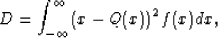 |
(1) |
where f(x) is the probability density function of the input signal. Consider the situation
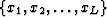
with L quantizers 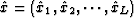 . Let the corresponding
quantization intervals be
. Let the corresponding
quantization intervals be
|  |
(2) |
where  and
and  . Then
|  |
(3) |
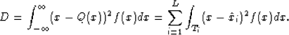
In the discrete case, equation (3) can be written as follows:
|  |
(4) |
where P(x) is the discrete version of the probability
density function, or normalized histogram ( ).
To minimize the distortion function D,
we take derivatives of equation (4) with
respect to
).
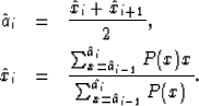
To minimize the distortion function D,
we take derivatives of equation (4) with
respect to  , ai and set them equal to zero,
leading to the following conditions for the optimum quantizers
and quantization interval boundaries
, ai and set them equal to zero,
leading to the following conditions for the optimum quantizers
and quantization interval boundaries  :
:
|  |
(5) |
| (6) |
A way to solve this coupled set of nonlinear equations is to first generate an initial set
 ,then apply equations (5) and (6) alternately until convergence is obtained.
This iteration is well known as the Lloyd-Max quantization algorithm (LMQ).
,then apply equations (5) and (6) alternately until convergence is obtained.
This iteration is well known as the Lloyd-Max quantization algorithm (LMQ).
It is fairly straightforward to extend the LMQ to 3D.
The main extension of the approach is to
break the input data points into 3D clusters instead of 1D cells. A 1D normalized histogram
should be replaced with a 3D normalized histogram and a 3D distortion
function should be calculated as follows:
| 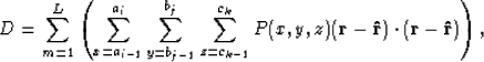 |
(7) |
where 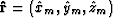 is the center of cluster m,
P(x,y,z) is the 3D histogram at point
is the center of cluster m,
P(x,y,z) is the 3D histogram at point  within cluster m, and
(ai-1,ai), (bj-1, bj), (ck-1, ck) define the boundaries of cluster m.
Conditions (5) and (6) accordingly become:
within cluster m, and
(ai-1,ai), (bj-1, bj), (ck-1, ck) define the boundaries of cluster m.
Conditions (5) and (6) accordingly become:
- 1.
- Classification of the points. The Euclidian distance between a point and every cluster center
(i.e. quantizer) is calculated. The
point is assigned to the closest cluster center.
- 2.
- Updating of the quantizers. Each quantizer is the center of mass of all points which are
assigned to the cluster.
It should be pointed out that LMQ is highly dependent on the initial
solution and can easily get stuck in local minima.
One simple but effective way to avoid these problems is to start with a uniform quantizer,
and when a cluster becomes empty, replace it by splitting regions with high variance Clapp (2004).
The detailed implementation of the modified
3D Lloyd's algorithm is discussed by Clapp (2006).
Next: selecting reference anisotropic parameters
Up: Tang and Clapp: Lloyd's
Previous: introduction
Stanford Exploration Project
4/5/2006