Gaussian pyramid generation

Suppose we start of with an initial image having N columns and M rows. This image forms the base or the zeroth level of the pyramid. Each point in the next level is computed as a weighted average of values in level within a 5-by-5 window, termed as the weighting function. The size of the weighting function is not critical in the pyramid generation process Burt (1981).

The pyramid generation process can now be represented as :  

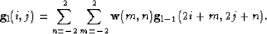$$\bold g_{\rm l}(i,j) = \sum_{n=-2}^2\sum_{m=-2}^2\bold w(m,n) \bold g_{\rm {l-1}}(2i+m,2j+n).$$ (1)

where w(m,n) is the weighting function. This same weighting function is used to generate the pyramid at each level. Notice that for each dimension the density of nodes is reduced by half from one level to the next.

The weighting function is chosen subject to certain constraints Burt (1981). For simplicity it is made separable:  

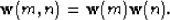$$\bold w(m,n) = \bold w(m) \bold w(n).$$ (2)

It is normalized to 1 and also made symmetric:  

$$\bold w(i) = \bold w(-i),\ \ \ i=0,1,2 .$$ (3)

It is also stipulated that each node contributes equally to nodes at the higher level so that a typical 5 point weighting function looks like:

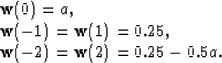$$\begin{array} {lll} \bold w(0) = a,\\ \bold w(-1) = \bold ... ... = 0.25,\\ \bold w(-2) = \bold w(2) = 0.25 - 0.5a. \end{array}$$ (4)

where a is a free parameter that controls the shape of the weighting function. For a = 0.4, the weighting function represents a Gaussian distribution in the limit.