SYN-1

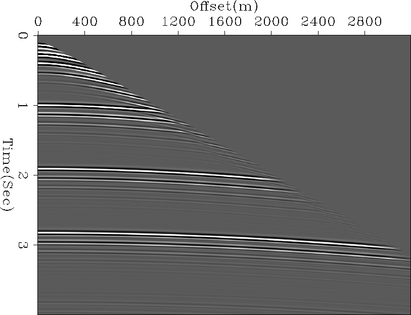
A synthetic data set, which we call SYN-1, was generated to simulate very shallow and hard water-bottom marine environment. The model has four horizontal layers. The depth of the water bottom is about 150 m. The data-set, shown in Figure , is contaminated with first- and higher-order water-bottom peglegs.

 

data
Figure 2 Synthetic data-set (SYN-1) infected with shallow water bottom multiples.

Brown (2004) discusses kinematic imaging of pegleg multiples and applies NMO correction for a j^th order pegleg using the following equation:  

$$t = \sqrt{ (\tau+j\tau^{*})^2 + \frac{x^2}{V_{\rm eff}^2} },$$ (9)

where $\tau$ and $\tau^{*}$ are the zero-offset travel-time and travel-time depth of the multiple generating surface respectively and $V_{\rm eff}$ is the effective velocity, which is given by  

$$V_{\rm eff}^2 = \frac{ \left( j\tau^* V_{\rm rms}^2(\tau^*) + \tau V_{\rm rms}^2(\tau) \right)}{\tau+j\tau^*}.$$ (10)

We use these kinematic equations in our NMO operator to construct images from primaries as well as from multiples. When we apply the NMO operator with V_rms as the velocity function, primaries get perfectly corrected for the moveout, but multiples have a residual moveout, and they appear as crosstalk. The same holds true for primaries and higher-order multiples when we correct with a $V_{\rm eff}$ appropriate for first-order multiples. Thus, in each image we should ideally be able to distinguish the components (primaries or different order of multiples) we correct for the moveout from others. These equations work fine for most cases, but for SYN-1 we actually evaluate a limiting case of these equations. In this case, the travel-time depth of the water bottom is very small, so for deeper layers we have

$${\tau^*} \ll {\tau}.$$ (11)

Using this in equations (9) and (10), we get  

$$t \Longrightarrow \sqrt{ \tau^2 + \frac{x^2}{V_{\rm eff}^2}},$$ (12)

 

$$V_{\rm eff} \Longrightarrow V_{rms}.$$ (13)

When we construct the image from primaries, we use V_rms to apply the NMO operator. In this case where V_rms $\approx$ $V_{\rm eff}$, we do not expect water-bottom peglegs to have a residual moveout. This is precisely the reason why in Figure all the primaries are imaged to their perfect positions, but the multiples, which we were expecting to appear as crosstalk, look like perfectly flat reflectors.

 

syn1i
Figure 3 Images constructed from (a) primary, (b) first- and (c) second-order multiples. A strong primary crosstalk is present on images constructed from first- and second-order multiples, moreover, its difficult to distinguish between signal and crosstalk on the basis of residual moveout.

Likewise, when we construct images from first- and higher-order multiples, we do not see any residual moveout for primaries and other multiples, except for shallow ones. In an ideal case, we would have a consistent signal across all the images, but the crosstalk would be inconsistent, a fact we could use to enhance signal-to-noise ratio and penalize crosstalk. But for this special case at hand, crosstalk is as consistent as the signal itself. LSJIMP uses three regularization operators as discussed in equation (8); two of these, differencing across offset (designed to penalize events with residual moveout) and differencing between images (designed to penalize inconsistent crosstalk) do not seem to work effectively for SYN-1. Moreover, the crosstalk-modeling operator fails to perfectly model the crosstalk and subsequently penalize the multiple energy. In Figure we can observe, a very strong primary crosstalk in images constructed from first- and second-order multiples.

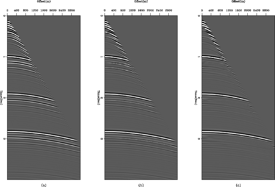
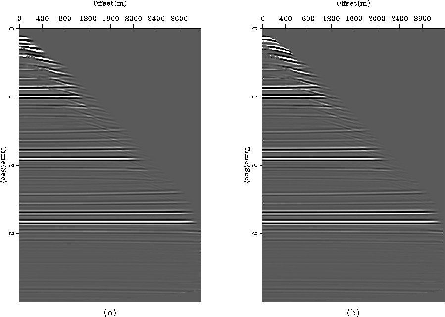
Thus, the application of LSJIMP to such a data set can indeed image the primaries but cannot eliminate water-bottom peglegs completely, as shown in Figure . Since most of the multiple energy present here is in water-bottom peglegs, we can use some simple tricks like predictive deconvolution to suppress this energy. We can also try to model the crosstalk by shifting the dataset by the travel-time depth of water bottom. The results for this exercise are given in Figure , though our results have improved a lot, we still have not been able to get rid of all the multiple energy in the shallow part(first-order water-bottom multiple). The primary reason is that most of the zone is muted, and we have few data points in that time range to perfectly model crosstalk.

The first regularizaton operator, $\bold r_m^{[1]}$ in equation 8, was a result of differencing between images of model panels generated by primaries and different orders of multiples. Ideally the difference between two of them should be small where signal is present and large where crosstalk dominates. Application of such a scheme ensures some degree of smoothness and consistency across images. 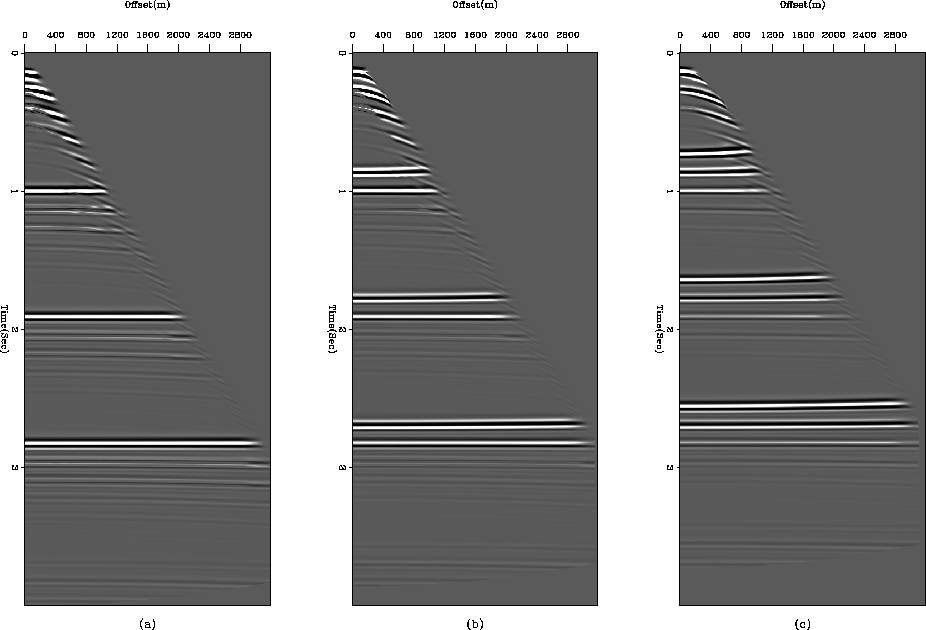LSJIMP computes the difference across two consecutive images, for instance between $\bold m_0$ and $\bold m_{101}$, $\bold m_{101}$ and $\bold m_{111}$ and likewise. Another possible alternative is to compute the difference between a multiple image and the primary image, as that would make all other images consistent with the primary, where we have maximum signal-to-noise ratio. We implemented this approach, but the results as given in Figure are not pleasing. The images we obtained have lots of ringing. One of the main reasons for this was the presence of strong primary crosstalk across all the panels which appears as a spurious event on the primary image after regularization.

 

syn1c1
Figure 4 Comparing (a) raw data (SYN-1) and (b) data generated by applying forward-modeling operator on primary image generated by LSJIMP

 

syn1c2
Figure 5 Comparing (a) raw data (SYN-1) and (b) data generated by applying forward-modeling operator on primary image generated by LSJIMP, and (c) LSJIMP with the modified crosstalk model. Notice the improvement in multiple suppression with modified LSJIMP.

 

regmod
Figure 6 Illustrating (a) primary image and (b) first-order multiple image with a revised regularization scheme. Notice the amount of ringing, and spurious events in primary image.