 |
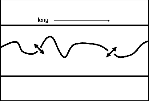
Figure 1 A cartoon of a masked salt boundary. It is long and thin with a discontinuous salt boundary snaking across it.
 |
Unfortunately, the normalized cut segmentation method tends to partition elongated images along their shortest dimension. For instance, Figure ![[*]](http://sepwww.stanford.edu/latex2html/cross_ref_motif.gif) is a cartoon of an elongated image with a salt boundary snaking across it. If the segmentation algorithm were to function as hoped, the minimum cut would be found along the salt boundary. However, because the salt boundary is discontinuous, it is likely that the minimum of the normalized cut in equation (1) will be found by cutting the image vertically where the image is thin.
is a cartoon of an elongated image with a salt boundary snaking across it. If the segmentation algorithm were to function as hoped, the minimum cut would be found along the salt boundary. However, because the salt boundary is discontinuous, it is likely that the minimum of the normalized cut in equation (1) will be found by cutting the image vertically where the image is thin.
To correct this problem, we exploit the fact that the upper boundary will necessarily be in Group A and the lower boundary will be in Group B. In other words, we want to force the segmentation algorithm to put the coarsely picked bounds in different groups.
We can enforce this constraint during the creation of the weight matrix (![]() ). Recall that this matrix contains weights relating each sample to other samples along paths within a neighborhood. For any given sample, if its search neighborhood happens to cross a coarse boundary, it becomes weighted to another sample at a random distance along the boundary. This can be imagined by wrapping the image on a globe so that both the upper and lower bounds collapse to points at the poles. When estimating the weight matrix, every time a path crosses the north or south pole, it continues down the other side. By implementing these ``Random'' boundaries, we are effectively removing the upper and lower boundaries.
). Recall that this matrix contains weights relating each sample to other samples along paths within a neighborhood. For any given sample, if its search neighborhood happens to cross a coarse boundary, it becomes weighted to another sample at a random distance along the boundary. This can be imagined by wrapping the image on a globe so that both the upper and lower bounds collapse to points at the poles. When estimating the weight matrix, every time a path crosses the north or south pole, it continues down the other side. By implementing these ``Random'' boundaries, we are effectively removing the upper and lower boundaries.
 |
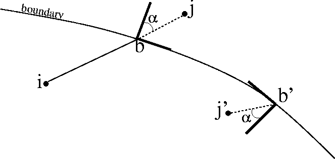
In Figure ![[*]](http://sepwww.stanford.edu/latex2html/cross_ref_motif.gif) , two nodes,
, two nodes, ![]() and
and ![]() , of a 2D image are plotted separated by a boundary indicating that node
, of a 2D image are plotted separated by a boundary indicating that node ![]() is outside of the bounds. Vector
is outside of the bounds. Vector ![]() represents the shortest path connecting them but excluding the nodes themselves.
represents the shortest path connecting them but excluding the nodes themselves. ![]() and
and ![]() are the unit normal and tangent vectors where
are the unit normal and tangent vectors where ![]() crosses the boundary at location
crosses the boundary at location ![]() . Together,
. Together, ![]() and
and ![]() , make a basis on to which vector
, make a basis on to which vector ![]() is projected and then mapped on to another basis at
is projected and then mapped on to another basis at ![]() at a random distance along the boundary. In summary, if
at a random distance along the boundary. In summary, if ![]() is outside the boundary, then
is outside the boundary, then ![]() defines the path instead of
defines the path instead of ![]() as:
as:
 |
(4) | |
| (5) | ||
| (6) |