Differential N-D Mesh Generation

Generalized Laplacian systems can be solved by many different ways; however, numerical solution often is facilitated through intermediate mappings to meshes exhibiting many attributes of the final grid. This consists of a composite of a transformation - $s^i(\xi^j)$ - from a Cartesian $\{ \xi^j \}$ to an intermediate basis $\{ s^i \}$, and a transformation - x^k(s^j) - from $\{ s^i \}$ to the final coordinate mesh $\{ x^k \}$. Notationally, the composite mapping transforms for the N-D problem are,

$$\begin{eqnarray} s^j(\xi^i) \; : \; \Xi^{n} \rightarrow S^{n},& \xi^i = \{ \xi^... ...\{ s^1, s^2, ... , s^n \} ,& x^k = \{ x^1, x^2, ... , x^{n+l} \}, \end{eqnarray}$$ (2)

Note that coordinate system $\{ x^k \}$ may be of a greater dimension than $\{ s^j \}$, which allows for composite mapping operations of $x^k \left[s^j \left(\xi^i \right)\right]\; : \; \Xi^n \rightarrow X^{n+k}$ that project a 2-D surface into 3-D space (see figure  for an example).

 

Example
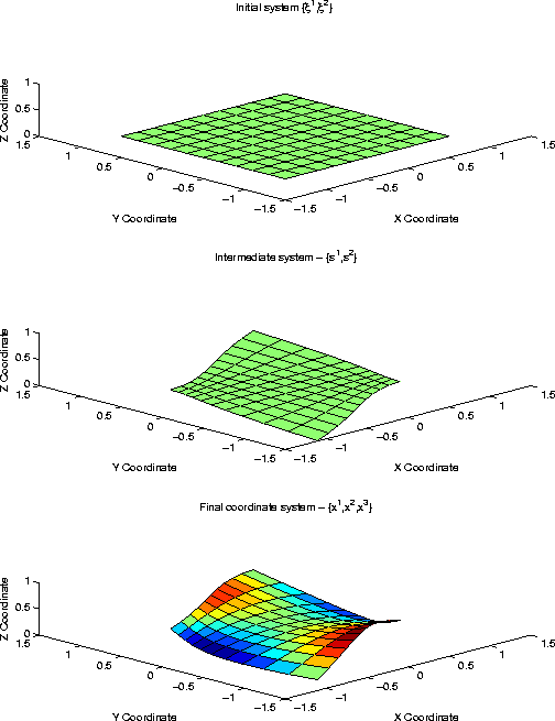
Figure 1 Meshing example for mapping a 2-D Cartesian domain to a surface in a 3-D volume. Top panel: Regular Cartesian mesh $\{ \xi^1,\xi^2 \}$; Middle panel: Intermediate transformation domain $\{ s^1,s^2 \}$; and Bottom panel: Surface in middle panel projected onto 3-D surface $\{ x^1,x^2,x^3 \}$ where increasing grey scale intensity represents increasing height.

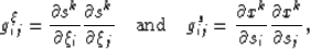
Coordinate system transformations - $s^j(\xi^i)$ and x^k(s^j) - are described in differential geometry through metric tensor, g_ij, which relates the geometry of a coordinate system $\{ s^j \}$ to that of $\{ \xi^i \}$ Guggenheimer (1977). The metric tensor is symmetric (i.e. g_ij=g_ji) and has elements given by,  

$$g^{\xi}_{ij} = \frac{\partial s^k}{\partial \xi_i} \frac{\pa... ...\partial x^k}{\partial s_i} \frac{\partial x^k}{\partial s_j},$$ (3)

where the metric tensor superscript specifies the coordinate system in which the operator is defined. (Note that summation notation - g_ii = g₁₁+g₂₂+g₃₃ - is implicit for any repeated indicies found in the paper.) The associated metric tensor g^ij is related to the metric tensor through g^ij = g_ij/|g^s| where g^s is the metric tensor determinant. Through use of this differential geometric framework, the governing set of differential gridding equations Liseikin (2004) become,

$$\begin{eqnarray} D^{\xi}[s^j] = \frac{1}{\sqrt{g_s} } \,\frac{\partial}{\partial... ...t\vert _{\partial S^n} = \phi^i \left[ s^j \right], \quad i,j=1,n.\end{eqnarray}$$ (4) (5)

Equations 4 represent the N generalized Laplace's equations acting on coordinate fields $\{ s^j \}$, and equations 5 map the boundary values of each coordinate field $\phi^i \left[s^j \right]$ to the boundary of domain $\Xi^n$. As posed, equations 4 and 5 provide no guarantee that generated grids will exhibit appropriate characteristics because no mesh regularization has yet been enforced.