A synthetic dataset for VTI media

Figures - show a synthetic model for a VTI medium. Figure shows the velocity model, Figure is the anisotropy parameter $\varepsilon$, and Figure is the anisotropy parameter $\delta$. There are 720 shots in total, and the maximum offset for each shot is 8000 meters. The challenging part of this model is to accurately image the steep fault, salt flank and the two abnormal sediments near the right corner of the salt body. I run plane-wave migration, using the extrapolation operator suggested by Shan and Biondi (2005). I generate 80 plane-wave sources, and the take-off angles at the surface range from $-40^\circ$ to $40^\circ$.

 

bprightnotilt
Figure 7 The image of the right salt body in Cartesian coordinates.

 

bprighttilt
Figure 8 The image of the right salt body in tilted coordinates.

 

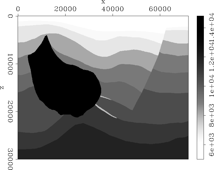
vpani
Figure 9 The vertical velocity model.

 

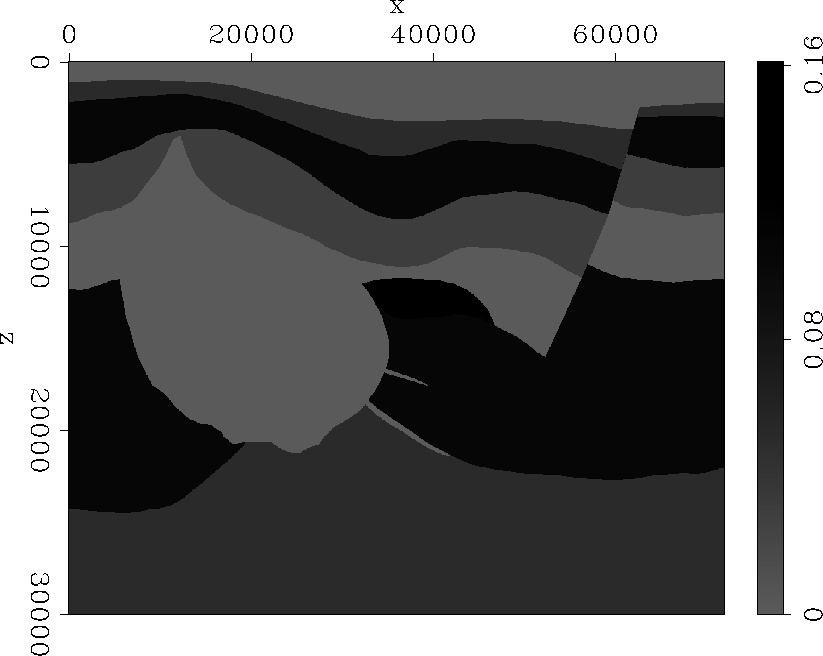
epsani
Figure 10 The anisotropy parameter $\varepsilon$.

 

dltani
Figure 11 The anisotropy parameter $\delta$.

 

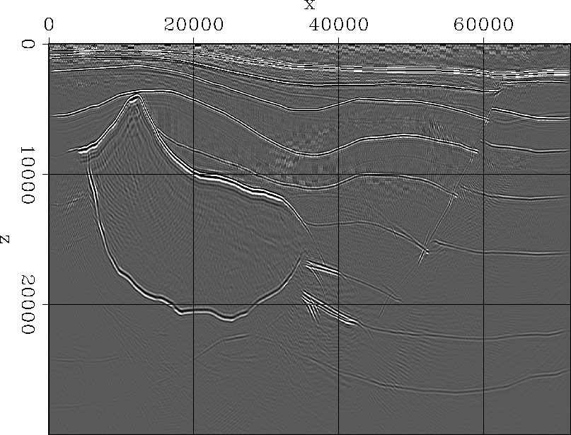
isohesstilt
Figure 12 Isotropic migration in tilted coordinates.

 

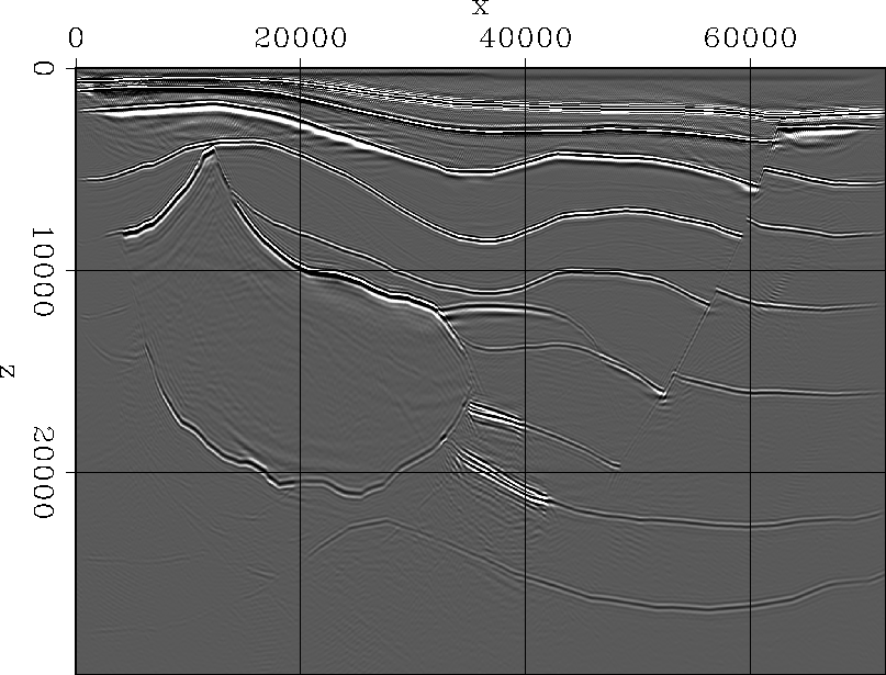
anihessnotilt
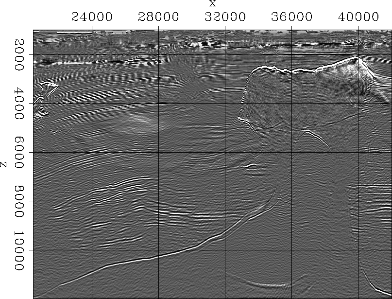
Figure 13 Anisotropic migration in Cartesian coordinates.

 

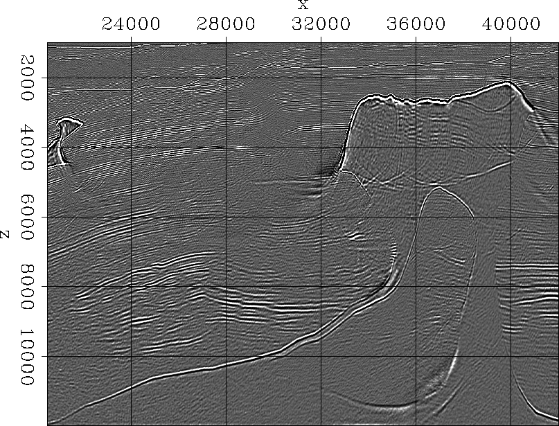
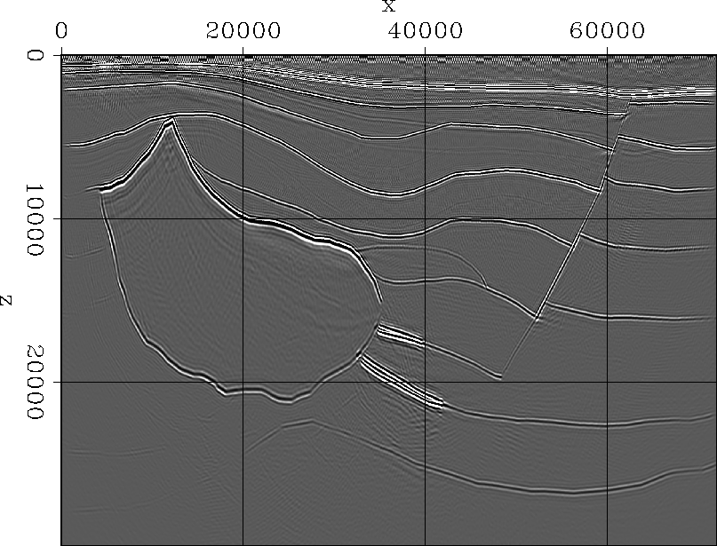
anihesstilt
Figure 14 Anisotropic migration in tilted coordinates.

 

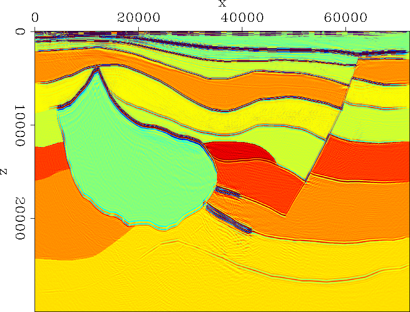
anihesstilteps
Figure 15 Anisotropic migration in tilted coordinates overlaid with the model.

Figure is the image obtained by isotropic plane-wave migration in tilted coordinates. Though we can see the energy of steeply dipping reflectors like the salt flanks and fault, they are not at the correct positions. Figure is the image obtained by anisotropic plane-wave migration in Cartesian coordinates. The reflectors are at the right positions, but some parts of the steeply dipping salt flank are lost, and the bottom of the fault is not well focused. Also the bottom abnormal sediment at the right corner of the salt body loses its energy where it is close to the salt. Figure is the image obtained by anisotropic plane-wave migration in tilted coordinates. In Figure , the salt flanks, the fault and abnormal sediments are all well imaged. Figure overlays the image by anisotropic plane-wave migration in tilted coordinates with the actual model, and shows that the reflectors are imaged at the correction positions.