 |
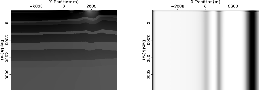
Figure 4 The left panel shows velocity field, the right panel shows the stretching of the coordinate system from Cartesian.
![[*]](http://sepwww.stanford.edu/latex2html/cross_ref_motif.gif) shows both the scaling of the orthogonal wave number (squeezing
and stretching of the coordinate system) and a velocity
component for the 2-D problem.
shows both the scaling of the orthogonal wave number (squeezing
and stretching of the coordinate system) and a velocity
component for the 2-D problem.
 |
At first glance these two fields do not show an obvious correlation.
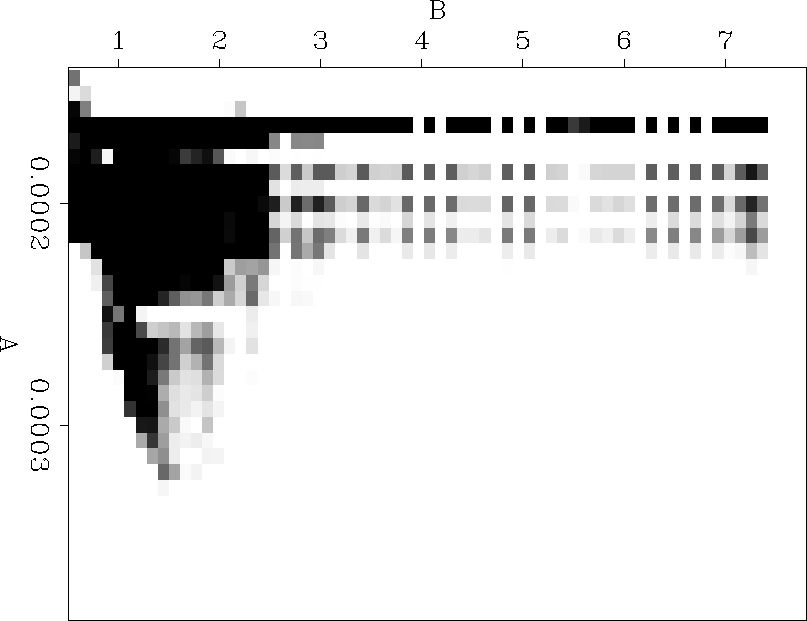
If we form a 2-D histogram (shown in Figure ![[*]](http://sepwww.stanford.edu/latex2html/cross_ref_motif.gif) ) another story emerges.
The parameters are correlated, and concentrated in top portion of the histogram.
Figure
) another story emerges.
The parameters are correlated, and concentrated in top portion of the histogram.
Figure ![[*]](http://sepwww.stanford.edu/latex2html/cross_ref_motif.gif) shows the histogram from several different
depths steps. The correlation and clustering of the parameters becomes even
more obvious. Figure
shows the histogram from several different
depths steps. The correlation and clustering of the parameters becomes even
more obvious. Figure ![[*]](http://sepwww.stanford.edu/latex2html/cross_ref_motif.gif) shows the
same depths overlaid by the N-D Lloyd codebook. Note how the histograms
features are easily identified. Figure
shows the
same depths overlaid by the N-D Lloyd codebook. Note how the histograms
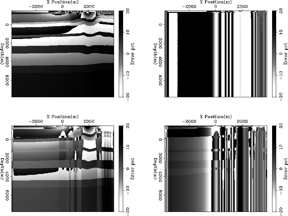
features are easily identified. Figure ![[*]](http://sepwww.stanford.edu/latex2html/cross_ref_motif.gif) shows
the error percentage in the parameters by using the N-D Lloyd approach
and by evenly partitioning the parameter range at each depth step. Not only is the
evenly spaced partitioning scheme eight times more expensive, the difference between
the true parameters at each model location and the selected parameters are
significantly higher. Tang and Clapp (2006) use a 3-D version of
Lloyd's algorithm for selected
shows
the error percentage in the parameters by using the N-D Lloyd approach
and by evenly partitioning the parameter range at each depth step. Not only is the
evenly spaced partitioning scheme eight times more expensive, the difference between
the true parameters at each model location and the selected parameters are
significantly higher. Tang and Clapp (2006) use a 3-D version of
Lloyd's algorithm for selected ![]() and
and ![]() parameters for anisotropic
migration.
parameters for anisotropic
migration.
|
jeff.histo
Figure 5 A 2-D histogram of the parameters shown in Figure ![[*]](http://sepwww.stanford.edu/latex2html/cross_ref_motif.gif) . The vertical axis
is velocity (A), the horizontal axis is the stretching parameter (B). The amplitude
shows the number of times a given (A,B) combination exists in the data shown
in Figure . The vertical axis
is velocity (A), the horizontal axis is the stretching parameter (B). The amplitude
shows the number of times a given (A,B) combination exists in the data shown
in Figure ![[*]](http://sepwww.stanford.edu/latex2html/cross_ref_motif.gif) . Note the correlation in the parameters. . Note the correlation in the parameters.
|  |
 |
 |
 |