


Next: Synthetic Examples
Up: Witten: Quaternion-based Signal Processing
Previous: Quaternionic Gabor Filters
Given two images, f1 and f2, it is possible to find a
vector field,  , that relates the local
displacement between f1 and
f2 (i.e.
, that relates the local
displacement between f1 and
f2 (i.e. 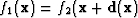 ).
Therefore, if the QFT of f1 is,
).
Therefore, if the QFT of f1 is,
| 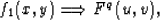 |
(17) |
then by the shift theorem,
|  |
(18) |
Knowing that f1 and f2 have local quaternionic phases
( ,
, ,
, ) and (
 ,
, ,
, ) and
assuming that
) and
assuming that  varies only in x and
  varies only in
y, then the displacement
varies only in
y, then the displacement  is given by
|  |
(19) |
| (20) |
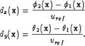
The accuracy of the displacement depends strongly on the choice of the
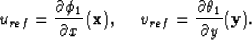
reference frequencies, uref and vref. The local model approach for quaternions
outlined by Bülow (1999) will be used. This model assumes that the local
phase at corresponding points of the two images will not differ,
 (x,y)=
 (x+dx,y+dy),
where
(x+dx,y+dy),
where  =(,). An estimate for
 is obtained by a first-order Taylor expansion of
  about x
|  |
(21) |
Solving for in equation 21 gives the disparity estimate
for the local model. The disparity is estimated using equation
19 and the reference frequencies given by,
|  |
(22) |
The local
quaternionic phase components for anywhere in an image are
given by
| 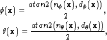 |
(23) |
| (24) |
where n and d are related to the rotation matrix of a quaternion
and are,
|  |
(25) |
| (26) |
| (27) |
| (28) |
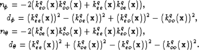
The k-functions are the responses of a symmetric component of the
quaternionic Gabor filter to the image (e.g. kee=(hee 
 ). From equations 23 and
24 the derivatives of the local phase components are computed
). From equations 23 and
24 the derivatives of the local phase components are computed
|  |
(29) |
| (30) |
Therefore, the disparity depends on the rate of change of the local
phase as approximated by the quaternionic Gabor filters.
Next: Synthetic Examples
Up: Witten: Quaternion-based Signal Processing
Previous: Quaternionic Gabor Filters
Stanford Exploration Project
4/5/2006