

Next: Future Work
Up: R. Clapp: Regularization
Previous: Implementation
I tested the methodology on a real 3-D marine dataset
from the North Sea. Figures ![[*]](http://sepwww.stanford.edu/latex2html/cross_ref_motif.gif) and
and ![[*]](http://sepwww.stanford.edu/latex2html/cross_ref_motif.gif) are from this dataset. Previous uses of AMO and common azimuth
migration have resulted in noticeable acquisition footprint
in the first 1000 meters Biondi (1999); Vaillant and Sava (1999).
For the test I used a maximum of 40 iterations, with a maximum reduction
in residual of 35%. A large reduction would be preferable but
many frequencies did not reduce by even 20% after 40 iterations.
Figure
are from this dataset. Previous uses of AMO and common azimuth
migration have resulted in noticeable acquisition footprint
in the first 1000 meters Biondi (1999); Vaillant and Sava (1999).
For the test I used a maximum of 40 iterations, with a maximum reduction
in residual of 35%. A large reduction would be preferable but
many frequencies did not reduce by even 20% after 40 iterations.
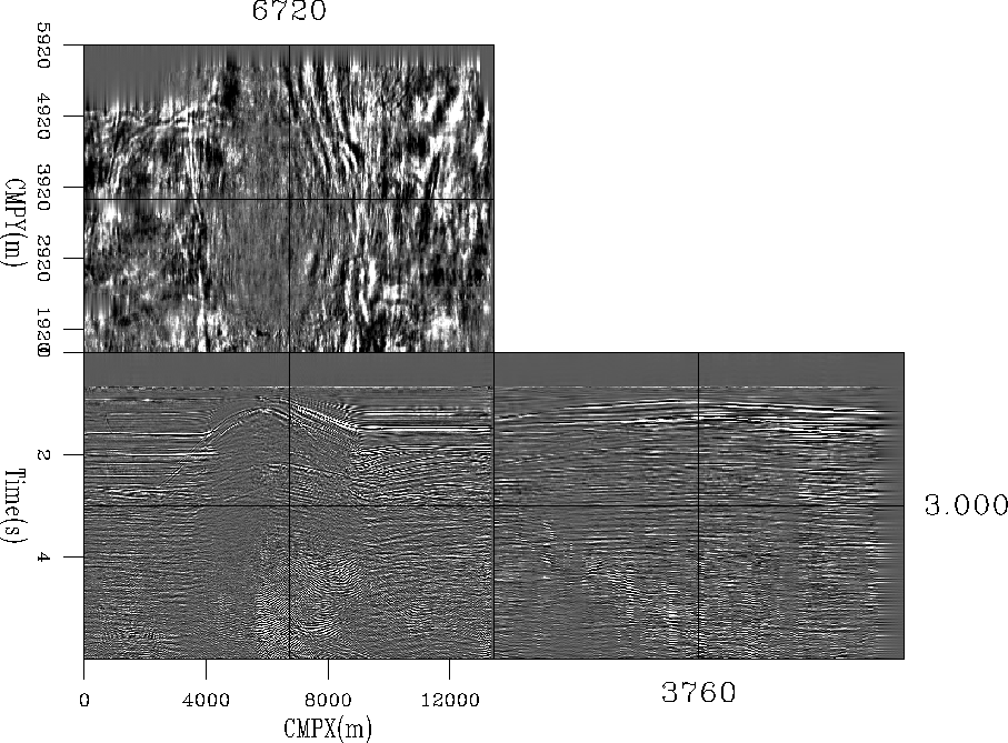
Figure ![[*]](http://sepwww.stanford.edu/latex2html/cross_ref_motif.gif) shows a constant offset section after
regularization with fitting goals (4). Note
the absence of an acquisition footprint. Further, note how
we have successfully filled even the large hole visible
in the fold map of Figure
shows a constant offset section after
regularization with fitting goals (4). Note
the absence of an acquisition footprint. Further, note how
we have successfully filled even the large hole visible
in the fold map of Figure ![[*]](http://sepwww.stanford.edu/latex2html/cross_ref_motif.gif) .
const-off
.
const-off
Figure 7 A constant offset section from a
real 3-D marine dataset obtained by applying fitting goals (4).
Note the absence of an acquisition footprint.


I then applied common azimuth migration to the data.
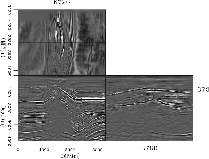
Figure ![[*]](http://sepwww.stanford.edu/latex2html/cross_ref_motif.gif) show three slices from the zero-offset
migration cube. Pay particular attention to the
depth slice. Note how the acquisition footprint has
disappeared.
show three slices from the zero-offset
migration cube. Pay particular attention to the
depth slice. Note how the acquisition footprint has
disappeared.
mig
Figure 8 The result of migrating the data show in
Figure ![[*]](http://sepwww.stanford.edu/latex2html/cross_ref_motif.gif) . Note that virtually no acquisition footprint
is visible in the data.
. Note that virtually no acquisition footprint
is visible in the data.


Next: Future Work
Up: R. Clapp: Regularization
Previous: Implementation
Stanford Exploration Project
10/31/2005

![[*]](http://sepwww.stanford.edu/latex2html/cross_ref_motif.gif) and
and ![[*]](http://sepwww.stanford.edu/latex2html/cross_ref_motif.gif) are from this dataset. Previous uses of AMO and common azimuth
migration have resulted in noticeable acquisition footprint
in the first 1000 meters Biondi (1999); Vaillant and Sava (1999).
For the test I used a maximum of 40 iterations, with a maximum reduction
in residual of 35%. A large reduction would be preferable but
many frequencies did not reduce by even 20% after 40 iterations.
Figure
are from this dataset. Previous uses of AMO and common azimuth
migration have resulted in noticeable acquisition footprint
in the first 1000 meters Biondi (1999); Vaillant and Sava (1999).
For the test I used a maximum of 40 iterations, with a maximum reduction
in residual of 35%. A large reduction would be preferable but
many frequencies did not reduce by even 20% after 40 iterations.
Figure ![[*]](http://sepwww.stanford.edu/latex2html/cross_ref_motif.gif) shows a constant offset section after
regularization with fitting goals (4). Note
the absence of an acquisition footprint. Further, note how
we have successfully filled even the large hole visible
in the fold map of Figure
shows a constant offset section after
regularization with fitting goals (4). Note
the absence of an acquisition footprint. Further, note how
we have successfully filled even the large hole visible
in the fold map of Figure ![[*]](http://sepwww.stanford.edu/latex2html/cross_ref_motif.gif) .
.

![[*]](http://sepwww.stanford.edu/latex2html/cross_ref_motif.gif) show three slices from the zero-offset
migration cube. Pay particular attention to the
depth slice. Note how the acquisition footprint has
disappeared.
show three slices from the zero-offset
migration cube. Pay particular attention to the
depth slice. Note how the acquisition footprint has
disappeared.

![[*]](http://sepwww.stanford.edu/latex2html/cross_ref_motif.gif) . Note that virtually no acquisition footprint
is visible in the data.
. Note that virtually no acquisition footprint
is visible in the data.