Next: Implementation
Up: Theory
Previous: Theory
This set of fitting goals can runs into problems when we deal with real
marine geometry.
To demonstrate the problem we will look at where data was recorded
for a real 3-D marine survey. We can calculate where we have traces in
the  plane. If our acquisition lines are perfectly straight,
we are able to acquire data throughout our survey. If our grid
is perfectly oriented with acquisition geometry, we should have consistent
fold in this cube. Figure
plane. If our acquisition lines are perfectly straight,
we are able to acquire data throughout our survey. If our grid
is perfectly oriented with acquisition geometry, we should have consistent
fold in this cube. Figure ![[*]](http://sepwww.stanford.edu/latex2html/cross_ref_motif.gif) shows that this is far from the case.
The figure shows the result of stacking over all offsets. Note that
we have some areas where we don't have any data (white).
If we use fitting goals (2) to estimate our model
we run into a problem.
The inversion result will show a dimming of amplitudes as we move
away from our known data.
shows that this is far from the case.
The figure shows the result of stacking over all offsets. Note that
we have some areas where we don't have any data (white).
If we use fitting goals (2) to estimate our model
we run into a problem.
The inversion result will show a dimming of amplitudes as we move
away from our known data.
fold
Figure 3 Fold of a real marine dataset. Note
how we have some regions with zero fold (white).
|
| 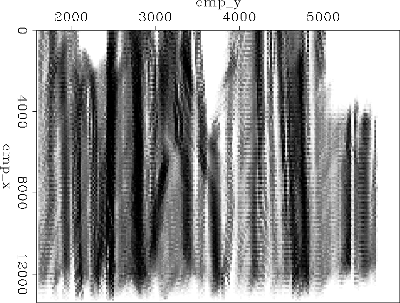 |


Figure shows the result of applying fitting goals (2)
to our synthetic. Note how the amplitude declines markedly as we move away
from locations where we have data.
Even more problematic than dimming is when we see significant
unrealistic, brightening of amplitudes for certain  . The brightening
is caused by the fold pattern
seen in Figure . The three panels represent
the fold in the (
. The brightening
is caused by the fold pattern
seen in Figure . The three panels represent
the fold in the ( ) plane as we increase in offset
from left to right. Note how we have fairly regular coverage at the near offsets
and much more variable coverage as we move to larger offsets.
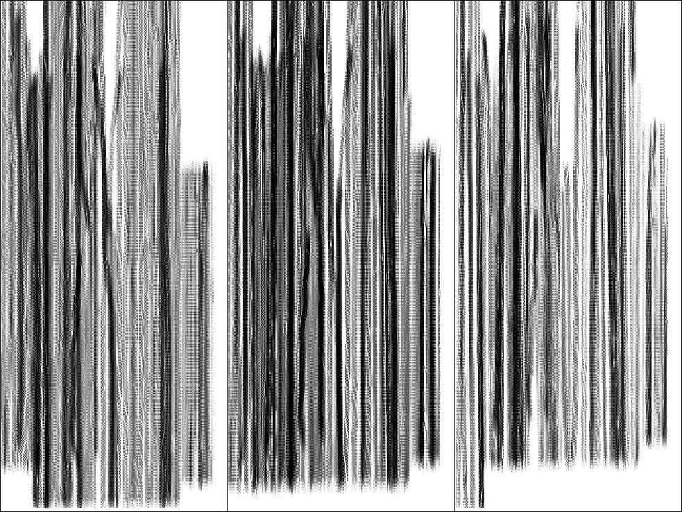
This inconsistency is mainly caused by cable feathering.
For some we only have near offset traces. The near offset traces tend to
be of higher amplitude and are more consistent as function of h
(the tops of hyperbolas are insensitive to velocity errors).
Our model covariance operator puts these unrealistically
large amplitudes at all offsets, resulting in a striping of the amplitudes
as a function of .
) plane as we increase in offset
from left to right. Note how we have fairly regular coverage at the near offsets
and much more variable coverage as we move to larger offsets.
This inconsistency is mainly caused by cable feathering.
For some we only have near offset traces. The near offset traces tend to
be of higher amplitude and are more consistent as function of h
(the tops of hyperbolas are insensitive to velocity errors).
Our model covariance operator puts these unrealistically
large amplitudes at all offsets, resulting in a striping of the amplitudes
as a function of .
fold-off
Figure 4 The three panels represent
the fold in the () plane as we increase in offset
from left to right. Note how we have fairly regular coverage at the near offsets
and much more variable coverage as we move to larger offsets.
For some we only have near offset traces.
bad-syn
Figure 5 Two views of the result of applying fitting goals (2).
The left panel is a three dimensional view at a fixed hx.
The right panel is a three dimensional view at a fixed  .Note the inconsistent, unrealistic amplitude behavior as a function of .
![[*]](http://sepwww.stanford.edu/latex2html/movie.gif)
Both of these problems are due to the lack of `mixing' of information
along the y direction.
By mixing I mean that
a column of the matrix implied by fitting goals ( ) has very few
non-zero elements at 's different from
the associated with its corresponding model point.
Our regularization is just DMO, which produces
no mixing in the y direction.
Our zeroing operator produces a limited amount of mixing,
but the range is limited due to the small offset in the hy direction
inherent in marine surveys.
As a result our inversion can have realistic kinematic but
unrealistic amplitude behavior as
a function of . A simple solution to this problem
is to introduce another operator to our model covariance
description that tends to produce consistency as
a function of . We must be careful to
avoid introducing unrealistic smoothness in the direction
by our choice of preconditioners.
I chose
leaky integration along
the plane
) has very few
non-zero elements at 's different from
the associated with its corresponding model point.
Our regularization is just DMO, which produces
no mixing in the y direction.
Our zeroing operator produces a limited amount of mixing,
but the range is limited due to the small offset in the hy direction
inherent in marine surveys.
As a result our inversion can have realistic kinematic but
unrealistic amplitude behavior as
a function of . A simple solution to this problem
is to introduce another operator to our model covariance
description that tends to produce consistency as
a function of . We must be careful to
avoid introducing unrealistic smoothness in the direction
by our choice of preconditioners.
I chose
leaky integration along
the plane  . The leaky integration will
encourage the inversion to keep consistent amplitudes unless
the data says otherwise. Using a relatively small
leaky parameter and a very small
. The leaky integration will
encourage the inversion to keep consistent amplitudes unless
the data says otherwise. Using a relatively small
leaky parameter and a very small  should
force it to have only an amplitude balancing effect rather
than an effect on the kinematics of the solution.
should
force it to have only an amplitude balancing effect rather
than an effect on the kinematics of the solution.
Combining our two model preconditioners we get a new operator  ,
,
|  |
(3) |
and a new set of fitting goals
|  |
(4) |
| |
Figure shows the result of applying fitting goals
(4) to the small synthetic. Note how the amplitude
behavior is much more consistent than the result shown in
Figure .
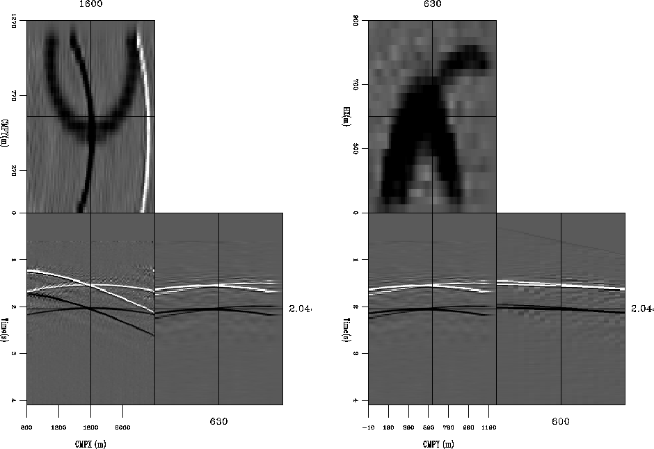
inv-syn
Figure 6 Two views of the result of applying fitting goals (4).
The left panel is a three dimensional view at a fixed hx.
The right panel is a three dimensional view at a fixed .Both views are identical the ones shown in Figure .
Note how the unrealistic amplitude behavior seen in Figure has
been corrected.
Fitting goals (4) should be avoided when possible.
They introduce a smoothing along the axis that is often
unrealistic. Unfortunately when encountering large acquisition
holes, some additional regularization is needed.
Next: Implementation
Up: Theory
Previous: Theory
Stanford Exploration Project
10/31/2005