Theory

Estimating a regularly sampled common-azimuth volume $\bf m$ from our irregular input data $\bf d$ can be set up as a least squares inversion problem. In this section, I will go over an approach to create a common azimuth volume by setting up an inverse problem. I will use a small synthetic to demonstrate the need for the various operators in the inversion process.

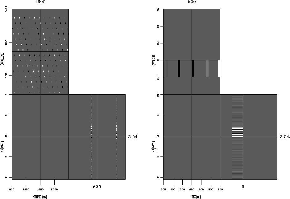
The data consists of irregular traces in a 5-D space ($t,{\rm cmp}_x, {\rm cmp}_y,h_x,h_y$). The AMO operator acts on regularly sampled ($t, {\rm cmp}_x, {\rm cmp}_y$) cubes, so we map from the irregular data space to the regular model space using a simple linear interpolation operator $\bf L$. Figure  shows two cube views from the five dimensional space the data is mapped into. Notice the sparseness of the data in these cubes. In standard marine acquisition, a single cross-line offset is acquired for each midpoint. The standard multi-streamer acquisition results in variation of the cross-line offset that is filled as we scan over ${\rm cmp}_y$.

 

interp Figure 1 The location of the input traces for a simple synthetic. The left panel is a constant offset cube (fixed hx and hy). The right panel is a single midpoint (fixed ${\rm cmp}_x$ and ${\rm cmp}_y$).

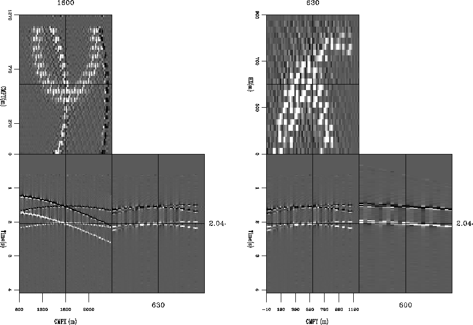
For common azimuth migration, we want all of our data to reside at h_y=0. As a result, we need to use AMO to transform from the h_y that the data was recorded at to h_y=0. The operator $\bf Z'$ is a sum over the ($t, {\rm cmp}_x, {\rm cmp}_y$) cubes that have been transformed to h_y=0. Figure  shows two cube views of the result of applying $\bf Z'$ to the small synthetic. In this case we still have significant holes along ${\rm cmp}_y$. I will discuss why I created these holes later in the section.

 

zero
Figure 2 The result of applying $\bf Z$ to the data shown in Figure . The left panel shows three slice from constant offset cube. The right panel shows three slice from a constant ${\rm cmp}_y$ cube.

Finally, we need to add in our regularization term. Generally, after NMO, our data should be smooth as a function of offset. We can think of adding a derivative operator along the offset axis. We can improve this estimate even further by applying a derivative on cubes that have been transformed to the same offset using AMO $\bf D_h$.We can write our fitting goals as

$$\begin{eqnarray} \bf d&\approx&\bf L\bf Z\bf m\\ \nonumber \bf 0&\approx&\epsilon \bf D_h\bf m,\end{eqnarray}$$ (1)

where $\epsilon$ controls the importance of consistency along the offset axis. We can speed up the convergence of this problem by preconditioning the model with the inverse of our regularization operator. In this case, we replace taking the derivative of AMO cubes with performing causal integration of AMO cubes $\bf C_h$. Our new fitting goals then become

$$\begin{eqnarray} \bf d&\approx&\bf L\bf Z\bf C_h\bf p \\ \nonumber \bf 0&\approx&\epsilon \bf p,\end{eqnarray}$$ (2)

where $\bf m= \bf C_h\bf p$.

 

• Large holes