

Next: Conclusion
Up: Synthetic and field data
Previous: Synthetic and field data
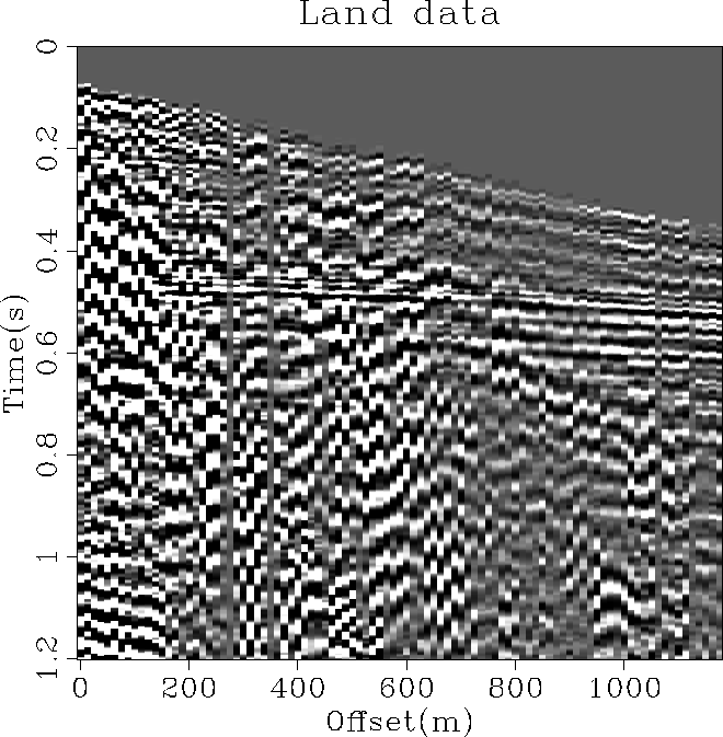
Figure ![[*]](http://sepwww.stanford.edu/latex2html/cross_ref_motif.gif) displays a CMP gather from a land
acquisition. This gather is contaminated by a strong ground-roll with
weak signal. The goal is to test the two proposed techniques with the
same operators as in the preceding example, i.e., hyperbolic radon
transform to obtain velocity information and a
displays a CMP gather from a land
acquisition. This gather is contaminated by a strong ground-roll with
weak signal. The goal is to test the two proposed techniques with the
same operators as in the preceding example, i.e., hyperbolic radon
transform to obtain velocity information and a  PEF
for the filtering and modeling of the noise.
amoco
Figure 7 A CMP gather from a land survey. The
ground-roll is very strong throughout the section.


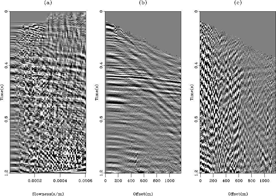
By doing inversion without taking care of the coherent noise,
the velocity panel in Figure ![[*]](http://sepwww.stanford.edu/latex2html/cross_ref_motif.gif) a is obtained.
The model space is contaminated with strong noise coming from
the residual in Figure
a is obtained.
The model space is contaminated with strong noise coming from
the residual in Figure ![[*]](http://sepwww.stanford.edu/latex2html/cross_ref_motif.gif) c.
When noise is present in the data, least-squares with a simple
damping can help to mitigate the noise effects. This was not done
in this case, however. The reconstructed data in Figure
c.
When noise is present in the data, least-squares with a simple
damping can help to mitigate the noise effects. This was not done
in this case, however. The reconstructed data in Figure
![[*]](http://sepwww.stanford.edu/latex2html/cross_ref_motif.gif) b is relatively noise free, which indicates that
most of the energy in the model space (Figure
b is relatively noise free, which indicates that
most of the energy in the model space (Figure ![[*]](http://sepwww.stanford.edu/latex2html/cross_ref_motif.gif) a)
is in the null space of the operator.
a)
is in the null space of the operator.
amoco-nopef
Figure 8 Result of least-squares inversion
of the data in Figure ![[*]](http://sepwww.stanford.edu/latex2html/cross_ref_motif.gif) . (a) Estimated model space.
The noise level is too high to see any useful information. (b) The
remodeled data. The low noise level in this panel indicates that most
of the energy in (a) resides in the null space of the operator. (c)
Data residual. The residual is not IID.
. (a) Estimated model space.
The noise level is too high to see any useful information. (b) The
remodeled data. The low noise level in this panel indicates that most
of the energy in (a) resides in the null space of the operator. (c)
Data residual. The residual is not IID.


For the filtering and modeling techniques to work, a noise model is
needed. As suggested in a preceding section, the noise model is
estimated from the residual of least-squares inversion assuming
that  (i.e., Figure
 ![[*]](http://sepwww.stanford.edu/latex2html/cross_ref_motif.gif) c).
From this noise model, a
c).
From this noise model, a  PEF is estimated.
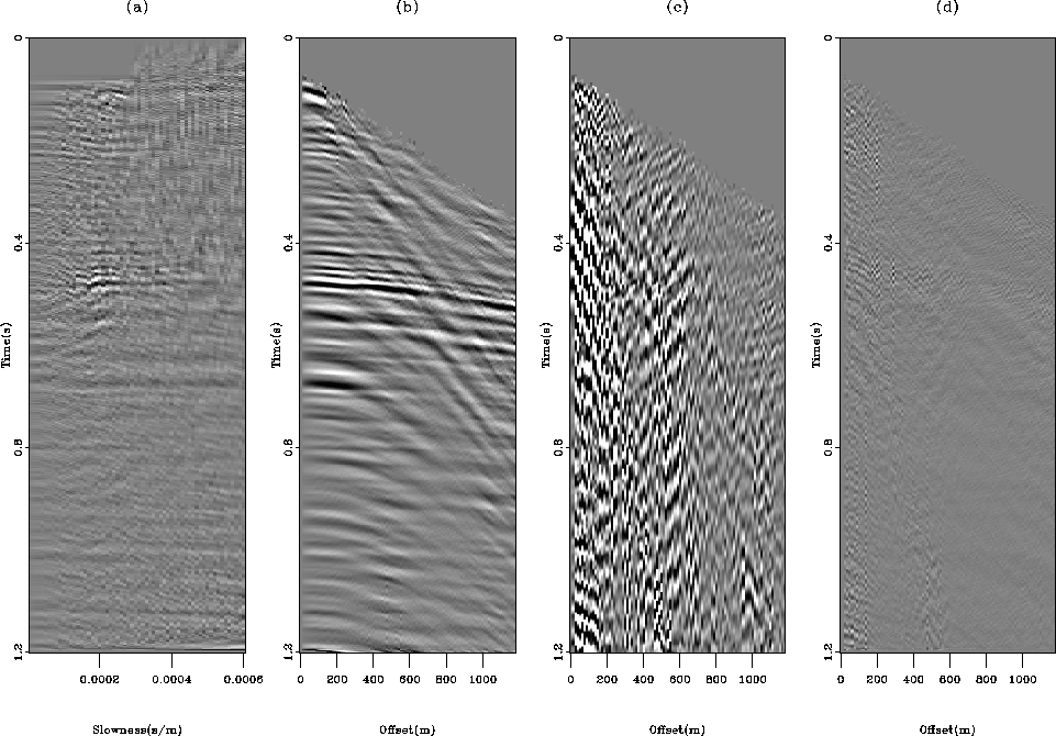
Figure
 ![[*]](http://sepwww.stanford.edu/latex2html/cross_ref_motif.gif) a displays the result of
the inversion after 40 iterations of CG. The few hyperbolas present
in the data are clearly mapped in the model space without any
artifact. The remodeled data in Figure
a displays the result of
the inversion after 40 iterations of CG. The few hyperbolas present
in the data are clearly mapped in the model space without any
artifact. The remodeled data in Figure ![[*]](http://sepwww.stanford.edu/latex2html/cross_ref_motif.gif) b show almost
no ground-roll remaining. The unweighted residual in Figure
b show almost
no ground-roll remaining. The unweighted residual in Figure
![[*]](http://sepwww.stanford.edu/latex2html/cross_ref_motif.gif) c (
c ( ) contains only coherent noise
and the residual in Figure
 ![[*]](http://sepwww.stanford.edu/latex2html/cross_ref_motif.gif) d is almost IID: a little
bit of ground-roll is still present.
d is almost IID: a little
bit of ground-roll is still present.
c-amoco
Figure 9 Inversion result with the filtering
technique.
(a) Estimated model.
(b) Remodeled data.
(c) Unweighted residual, showing the ground-roll only.
(d) Residual. The residual is not exactly IID. Some coherent
energy remains.


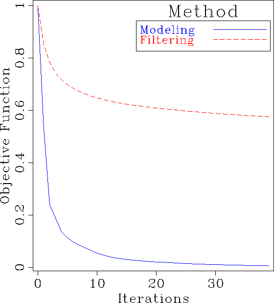
The modeling technique leads to similar results to the filtering
technique, as shown in Figure ![[*]](http://sepwww.stanford.edu/latex2html/cross_ref_motif.gif) . The main difference
comes from the residual in Figure
. The main difference
comes from the residual in Figure ![[*]](http://sepwww.stanford.edu/latex2html/cross_ref_motif.gif) d. With the modeling
method, the residual is smaller than with the filtering technique and
is IID. As a final comparison between the two techniques, Figure
d. With the modeling
method, the residual is smaller than with the filtering technique and
is IID. As a final comparison between the two techniques, Figure
![[*]](http://sepwww.stanford.edu/latex2html/cross_ref_motif.gif) shows how the objective function (normalized)
decreases in both cases. The modeling technique has the best
convergence properties.
shows how the objective function (normalized)
decreases in both cases. The modeling technique has the best
convergence properties.
compsa
Figure 10 Inversion result with the modeling
technique.
(a) Estimated model  .
(b) Remodeled data
  .(c) Remodeled noise
  .(d) Residual. The residual is IID.


amococonv
Figure 11 A comparison of convergence between
the filtering and modeling approach for the land data example.
|
|  |


Next: Conclusion
Up: Synthetic and field data
Previous: Synthetic and field data
Stanford Exploration Project
5/5/2005
![[*]](http://sepwww.stanford.edu/latex2html/cross_ref_motif.gif) displays a CMP gather from a land
acquisition. This gather is contaminated by a strong ground-roll with
weak signal. The goal is to test the two proposed techniques with the
same operators as in the preceding example, i.e., hyperbolic radon
transform to obtain velocity information and a
displays a CMP gather from a land
acquisition. This gather is contaminated by a strong ground-roll with
weak signal. The goal is to test the two proposed techniques with the
same operators as in the preceding example, i.e., hyperbolic radon
transform to obtain velocity information and a 
![[*]](http://sepwww.stanford.edu/latex2html/cross_ref_motif.gif) a is obtained.
The model space is contaminated with strong noise coming from
the residual in Figure
a is obtained.
The model space is contaminated with strong noise coming from
the residual in Figure ![[*]](http://sepwww.stanford.edu/latex2html/cross_ref_motif.gif) c.
When noise is present in the data, least-squares with a simple
damping can help to mitigate the noise effects. This was not done
in this case, however. The reconstructed data in Figure
c.
When noise is present in the data, least-squares with a simple
damping can help to mitigate the noise effects. This was not done
in this case, however. The reconstructed data in Figure
![[*]](http://sepwww.stanford.edu/latex2html/cross_ref_motif.gif) b is relatively noise free, which indicates that
most of the energy in the model space (Figure
b is relatively noise free, which indicates that
most of the energy in the model space (Figure ![[*]](http://sepwww.stanford.edu/latex2html/cross_ref_motif.gif) a)
is in the null space of the operator.
a)
is in the null space of the operator.
![[*]](http://sepwww.stanford.edu/latex2html/cross_ref_motif.gif) . (a) Estimated model space.
The noise level is too high to see any useful information. (b) The
remodeled data. The low noise level in this panel indicates that most
of the energy in (a) resides in the null space of the operator. (c)
Data residual. The residual is not IID.
. (a) Estimated model space.
The noise level is too high to see any useful information. (b) The
remodeled data. The low noise level in this panel indicates that most
of the energy in (a) resides in the null space of the operator. (c)
Data residual. The residual is not IID.
![]() (i.e., Figure
(i.e., Figure ![[*]](http://sepwww.stanford.edu/latex2html/cross_ref_motif.gif) c).
From this noise model, a
c).
From this noise model, a ![]() PEF is estimated.
Figure
PEF is estimated.
Figure ![[*]](http://sepwww.stanford.edu/latex2html/cross_ref_motif.gif) a displays the result of
the inversion after 40 iterations of CG. The few hyperbolas present
in the data are clearly mapped in the model space without any
artifact. The remodeled data in Figure
a displays the result of
the inversion after 40 iterations of CG. The few hyperbolas present
in the data are clearly mapped in the model space without any
artifact. The remodeled data in Figure ![[*]](http://sepwww.stanford.edu/latex2html/cross_ref_motif.gif) b show almost
no ground-roll remaining. The unweighted residual in Figure
b show almost
no ground-roll remaining. The unweighted residual in Figure
![[*]](http://sepwww.stanford.edu/latex2html/cross_ref_motif.gif) c (
c (![]() ) contains only coherent noise
and the residual in Figure
) contains only coherent noise
and the residual in Figure ![[*]](http://sepwww.stanford.edu/latex2html/cross_ref_motif.gif) d is almost IID: a little
bit of ground-roll is still present.
d is almost IID: a little
bit of ground-roll is still present.

![[*]](http://sepwww.stanford.edu/latex2html/cross_ref_motif.gif) . The main difference
comes from the residual in Figure
. The main difference
comes from the residual in Figure ![[*]](http://sepwww.stanford.edu/latex2html/cross_ref_motif.gif) d. With the modeling
method, the residual is smaller than with the filtering technique and
is IID. As a final comparison between the two techniques, Figure
d. With the modeling
method, the residual is smaller than with the filtering technique and
is IID. As a final comparison between the two techniques, Figure
![[*]](http://sepwww.stanford.edu/latex2html/cross_ref_motif.gif) shows how the objective function (normalized)
decreases in both cases. The modeling technique has the best
convergence properties.
shows how the objective function (normalized)
decreases in both cases. The modeling technique has the best
convergence properties.
