

Next: Land data example
Up: Noise attenuation by filtering
Previous: From filtering to covariance-pattern
Figure ![[*]](http://sepwww.stanford.edu/latex2html/cross_ref_motif.gif) a displays a synthetic CMP gather
composed of hyperbolas (the signal) and a monochromatic plane-wave
(the noise). The true signal and noise are shown in Figures
a displays a synthetic CMP gather
composed of hyperbolas (the signal) and a monochromatic plane-wave
(the noise). The true signal and noise are shown in Figures
![[*]](http://sepwww.stanford.edu/latex2html/cross_ref_motif.gif) b and
b and ![[*]](http://sepwww.stanford.edu/latex2html/cross_ref_motif.gif) c with their (f,k)
spectra. It is interesting to notice that the noise and signal overlap
in the (f,k) domain. This can be seen in the CMP gather
where the noise has (1) similar dips to some hyperbola tails, and (2) similar
frequency content. This overlap makes signal preservation particularly
difficult to achieve with simple filtering techniques such as bandpass.
datasynth
c with their (f,k)
spectra. It is interesting to notice that the noise and signal overlap
in the (f,k) domain. This can be seen in the CMP gather
where the noise has (1) similar dips to some hyperbola tails, and (2) similar
frequency content. This overlap makes signal preservation particularly
difficult to achieve with simple filtering techniques such as bandpass.
datasynth
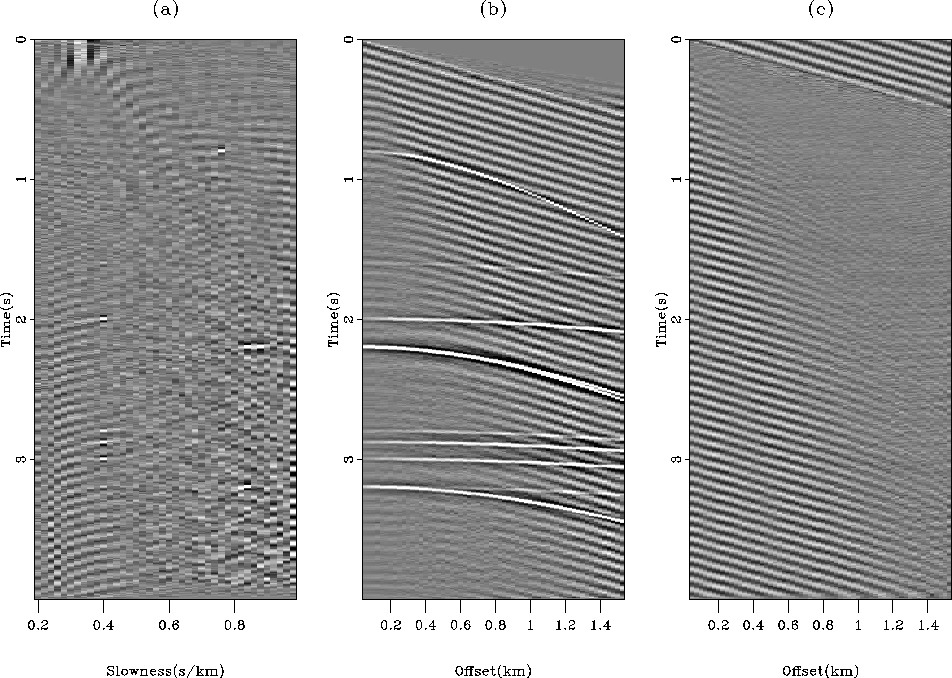
Figure 2 A synthetic data example with (a)
the data and its (f,k) spectrum, (b) the true signal and its (f,k)
spectrum, and (c) the noise. The spectra of signal and the noise
overlap, which makes simple filtering (i.e., without inversion)
likely to fail.


From this dataset, the goal is to estimate in a least-squares sense
a velocity panel with the hyperbolic radon
transform of Chapter ![[*]](http://sepwww.stanford.edu/latex2html/cross_ref_motif.gif) (
( ). This velocity
panel can be later used for velocity analysis or multiple attenuation
Alvarez and Larner (2004); Foster and Mosher (1992); Thorson and Claerbout (1985).
A conjugate-gradient (CG) solver is used for the iterations.
Figure
 ![[*]](http://sepwww.stanford.edu/latex2html/cross_ref_motif.gif) a illustrates the effects of the coherent
noise on the model space after inversion of the data in Figure
a illustrates the effects of the coherent
noise on the model space after inversion of the data in Figure
![[*]](http://sepwww.stanford.edu/latex2html/cross_ref_motif.gif) a. Some energy corresponding to both
the signal and the noise is present in Figure
a. Some energy corresponding to both
the signal and the noise is present in Figure ![[*]](http://sepwww.stanford.edu/latex2html/cross_ref_motif.gif) a,
but overall, it is quite difficult to recognize events corresponding
to the signal. The remodeled data in Figure
a,
but overall, it is quite difficult to recognize events corresponding
to the signal. The remodeled data in Figure ![[*]](http://sepwww.stanford.edu/latex2html/cross_ref_motif.gif) b
(i.e.,
b
(i.e.,  ) indicate that the inversion is fitting
both the noise and signal, which creates artifacts in
Figure
 ![[*]](http://sepwww.stanford.edu/latex2html/cross_ref_motif.gif) a. In addition, note that the residual (i.e.,
a. In addition, note that the residual (i.e.,  ) in Figure
 ![[*]](http://sepwww.stanford.edu/latex2html/cross_ref_motif.gif) c is not IID: a lot
of coherent energy remains. Therefore, the filtering and modeling
techniques are needed to obtain (1) IID residuals, (2) a better
velocity panel, and (3) noise-free remodeled data.
c is not IID: a lot
of coherent energy remains. Therefore, the filtering and modeling
techniques are needed to obtain (1) IID residuals, (2) a better
velocity panel, and (3) noise-free remodeled data.
synth-nopef
Figure 3 (a) Estimated model space after
inversion of the noisy data in Figure ![[*]](http://sepwww.stanford.edu/latex2html/cross_ref_motif.gif) a. (b)
Remodeled data from the inverted model. (c) Residual
a. (b)
Remodeled data from the inverted model. (c) Residual  after inversion. The residual is not IID and a lot of noise
contaminates the model space.


In this example, the noise is assumed to be known. For the filtering
approach, a  PEF is used for
  in
equation (
in
equation (![[*]](http://sepwww.stanford.edu/latex2html/cross_ref_motif.gif) ). For the modeling approach,
). For the modeling approach,  and
and
 ,
,  being the same PEF that for the
filtering approach.
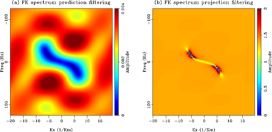
First, as an illustration on how a simple
prediction-filter differs from a projection filter, Figure
![[*]](http://sepwww.stanford.edu/latex2html/cross_ref_motif.gif) a displays the spectrum of the PEF
a displays the spectrum of the PEF  only and
Figure
 ![[*]](http://sepwww.stanford.edu/latex2html/cross_ref_motif.gif) b the spectrum of the projection
filter
b the spectrum of the projection
filter  with
with  .The PEF is estimated from the known noise, and we notice that its
spectrum in Figure
 ![[*]](http://sepwww.stanford.edu/latex2html/cross_ref_motif.gif) a is the smallest at the noise
location. The amplitude varies a lot with local minima and a
maximum amplitude far from one, however. The spectrum
of the projection filter in Figure
a is the smallest at the noise
location. The amplitude varies a lot with local minima and a
maximum amplitude far from one, however. The spectrum
of the projection filter in Figure ![[*]](http://sepwww.stanford.edu/latex2html/cross_ref_motif.gif) b is better behaved:
it equals zero at the noise location and is flat almost everywhere.
The maximum energy is not exactly one because a damping term was added
for the division.
b is better behaved:
it equals zero at the noise location and is flat almost everywhere.
The maximum energy is not exactly one because a damping term was added
for the division.
pefs
Figure 4 (a) (f,k) spectrum of the PEF. It is
minimum at the noise location but varies a lot everywhere else.
(b) (f,k) spectrum of the projection filter. It is minimum at the noise
location and flat otherwise. The projection filter is a better filter
than the prediction filter.


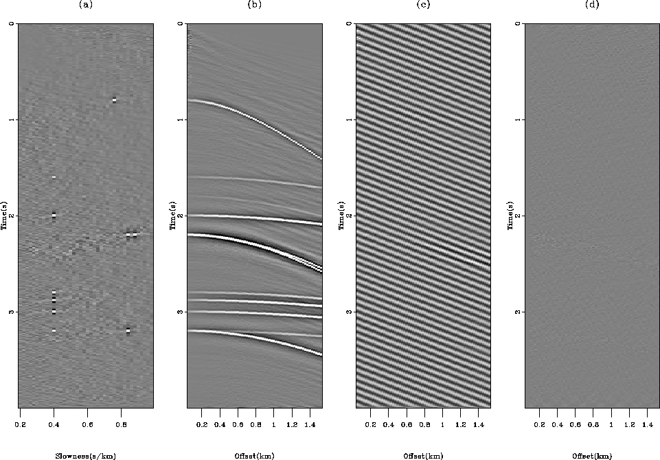
Figure ![[*]](http://sepwww.stanford.edu/latex2html/cross_ref_motif.gif) displays the result of the inversion with the
filtering approach. The estimated model in Figure
displays the result of the inversion with the
filtering approach. The estimated model in Figure ![[*]](http://sepwww.stanford.edu/latex2html/cross_ref_motif.gif) a
is now noise-free and the hyperbolas are well focused in the velocity
space. The residual in Figure
a
is now noise-free and the hyperbolas are well focused in the velocity
space. The residual in Figure ![[*]](http://sepwww.stanford.edu/latex2html/cross_ref_motif.gif) d has no coherent
energy left and is IID. The remodeled data in Figure
d has no coherent
energy left and is IID. The remodeled data in Figure
![[*]](http://sepwww.stanford.edu/latex2html/cross_ref_motif.gif) b are also basically noise free, and so is the
unweighted residual (
b are also basically noise free, and so is the
unweighted residual ( ) in Figure
 ![[*]](http://sepwww.stanford.edu/latex2html/cross_ref_motif.gif) c.
Therefore, the filtering technique worked very well and delivered the
expected results.
c.
Therefore, the filtering technique worked very well and delivered the
expected results.
c-synth
Figure 5 Inversion result with the filtering
technique.
(a) Estimated model.
(b) Remodeled data.
(c) Unweighted residual, which shows the coherent noise only.
(d) Residual. The estimated model is artifacts free and the residual
is IID. The movie shows the four panel as a function of the
iterations.


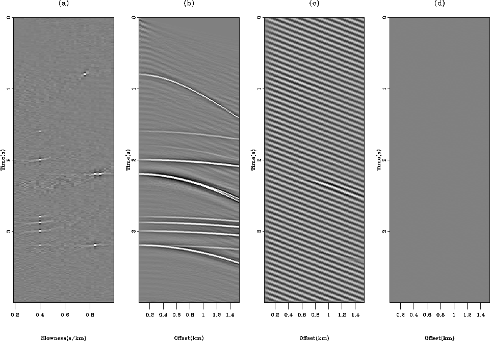
Figure ![[*]](http://sepwww.stanford.edu/latex2html/cross_ref_motif.gif) shows the result of the modeling
approach. Remember that the inverse of the
shows the result of the modeling
approach. Remember that the inverse of the  PEF estimated
from the true noise is used for the noise operator
  and that the hyperbolic radon transform is used to model
the signal. The balancing parameter
  in equation
(
in equation
(![[*]](http://sepwww.stanford.edu/latex2html/cross_ref_motif.gif) ) is chosen by trial and error.
) is chosen by trial and error.
The estimated model after inversion is shown in Figure
![[*]](http://sepwww.stanford.edu/latex2html/cross_ref_motif.gif) a. Similar to what we observed with the filtering
approach, the model is noise free and easy to interpret. The remodeled
data in Figure
a. Similar to what we observed with the filtering
approach, the model is noise free and easy to interpret. The remodeled
data in Figure ![[*]](http://sepwww.stanford.edu/latex2html/cross_ref_motif.gif) b show a little bit of coherent noise.
The problem stems from the fact that the two modeling operators
overlap: the inverse PEF can model some tails of hyperbolas and
the radon transform can fit some of the coherent noise
(because the velocity of the noise is within the range of the slowness
scan). Although not crucial here, a regularization term would improve
this result Nemeth (1996). The estimated noise of Figure
b show a little bit of coherent noise.
The problem stems from the fact that the two modeling operators
overlap: the inverse PEF can model some tails of hyperbolas and
the radon transform can fit some of the coherent noise
(because the velocity of the noise is within the range of the slowness
scan). Although not crucial here, a regularization term would improve
this result Nemeth (1996). The estimated noise of Figure
![[*]](http://sepwww.stanford.edu/latex2html/cross_ref_motif.gif) c proves that the separation worked very well. A
little bit of one hyperbola has been absorbed, however. The residual
in Figure
c proves that the separation worked very well. A
little bit of one hyperbola has been absorbed, however. The residual
in Figure ![[*]](http://sepwww.stanford.edu/latex2html/cross_ref_motif.gif) d is IID which confirms that the goals
of this technique were reached.
d is IID which confirms that the goals
of this technique were reached.
compsy
Figure 6 Inversion result with the modeling
technique.
(a) Estimated model  .
(b) Remodeled data
  .(c) Remodeled noise
  .(d) Residual. The residual is IID and the model space is
clean. Because the signal and noise modeling operators tend to
overlap, a little bit of noise leaks in the estimated signal. This
effect is very small, however.


![[*]](http://sepwww.stanford.edu/latex2html/cross_ref_motif.gif) a displays a synthetic CMP gather
composed of hyperbolas (the signal) and a monochromatic plane-wave
(the noise). The true signal and noise are shown in Figures
a displays a synthetic CMP gather
composed of hyperbolas (the signal) and a monochromatic plane-wave
(the noise). The true signal and noise are shown in Figures


