

Next: Regularization of the filter
Up: Estimation of nonstationary PEFs
Previous: Definitions
When PEFs are estimated, the matrix  is unknown. If
  is the data vector from which we want to estimate the filters, we
minimize the vector
  as follows:
|  |
(125) |
which can be rewritten
|  |
(126) |
where  is the matrix representation of the non-stationary
convolution or combination with the input vector
  .The transition between equations (
![[*]](http://sepwww.stanford.edu/latex2html/cross_ref_motif.gif) ) and (
) and (![[*]](http://sepwww.stanford.edu/latex2html/cross_ref_motif.gif) )
is not simple. In particular, the shape of the matrix
)
is not simple. In particular, the shape of the matrix  is
quite different if we are doing non-stationary convolution or
combination. For the convolution, we have
|  |
(127) |

We see that for the convolution case, the  matrices
are diagonal operators, translating the need for one filter to be
applied to one input point. The size of the matrix
  is
is
 where nf is the number of filter
coefficients.
Now, for the combination, we have
|  |
(128) |

We see that for the combination case, the  matrices
are row operators, translating the need for one filter to be
constant for one output point. The size of
  is equal to
the size of
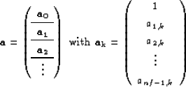
  .For the vector
  in equation (
![[*]](http://sepwww.stanford.edu/latex2html/cross_ref_motif.gif) ) we have
) we have
|  |
(129) |
where nf is the number of coefficients per filter. This definition
of  is independent of
  .We might want to have one filter common to different input or
output points instead of one filter per point. In that case, the
matrix
  is obtained by adding successive
  matrices
depending on how many points have a similar filter.
Note that in the stationary case, for both the convolution and the
combination case we have
 and
and
|  |
(130) |
Therefore, for the matrix  , we have to add all the
  matrices together. If we take advantage of the
special structure of
  for the convolution and the
combination, we obtain for the stationary case
| 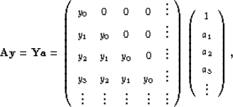 |
(131) |
which is the matrix formulation of the stationary convolution.
With the definitions given in equations
(![[*]](http://sepwww.stanford.edu/latex2html/cross_ref_motif.gif) ), (
), (![[*]](http://sepwww.stanford.edu/latex2html/cross_ref_motif.gif) ) and (
) and (![[*]](http://sepwww.stanford.edu/latex2html/cross_ref_motif.gif) ), the fitting goal in
equation (
), the fitting goal in
equation (![[*]](http://sepwww.stanford.edu/latex2html/cross_ref_motif.gif) ) can be rewritten
) can be rewritten
|  |
(132) |
or
|  |
(133) |
Each vector  has one constrained coefficient. We can then
rewrite equations (
has one constrained coefficient. We can then
rewrite equations (![[*]](http://sepwww.stanford.edu/latex2html/cross_ref_motif.gif) ) and (
) and (![[*]](http://sepwww.stanford.edu/latex2html/cross_ref_motif.gif) ) as follows:
) as follows:
|  |
(134) |
and
|  |
(135) |
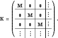
with
| 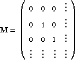 |
(136) |
The definition of  assumes that the first coefficient of each
filter is known. Note that
  is equal for both convolution and
combination methods.
Having defined the matrix
  , we can now rewrite
equation (
, we can now rewrite
equation (![[*]](http://sepwww.stanford.edu/latex2html/cross_ref_motif.gif) ) as follows:
) as follows:
|  |
(137) |
where the square matrix  is
is
|  |
(138) |
The next step consists of estimating the filter coefficients in a
least-squares sense.


Next: Regularization of the filter
Up: Estimation of nonstationary PEFs
Previous: Definitions
Stanford Exploration Project
5/5/2005
![[*]](http://sepwww.stanford.edu/latex2html/cross_ref_motif.gif) ) and (
) and (![[*]](http://sepwww.stanford.edu/latex2html/cross_ref_motif.gif) )
is not simple. In particular, the shape of the matrix
)
is not simple. In particular, the shape of the matrix 

![[*]](http://sepwww.stanford.edu/latex2html/cross_ref_motif.gif) ) we have
) we have


![[*]](http://sepwww.stanford.edu/latex2html/cross_ref_motif.gif) ), (
), (![[*]](http://sepwww.stanford.edu/latex2html/cross_ref_motif.gif) ) and (
) and (![[*]](http://sepwww.stanford.edu/latex2html/cross_ref_motif.gif) ), the fitting goal in
equation (
), the fitting goal in
equation (![[*]](http://sepwww.stanford.edu/latex2html/cross_ref_motif.gif) ) can be rewritten
) can be rewritten
![[*]](http://sepwww.stanford.edu/latex2html/cross_ref_motif.gif) ) and (
) and (![[*]](http://sepwww.stanford.edu/latex2html/cross_ref_motif.gif) ) as follows:
) as follows:

![[*]](http://sepwww.stanford.edu/latex2html/cross_ref_motif.gif) ) as follows:
) as follows:
