Elliptical Anisotropy

In this section, we derive the Common Azimuth downward continuation operator for an elliptically anisotropic media. The 3-D dispersion relation for VTI media given by Alkhalifah (1998) is:  

$$k_z = \frac{\omega}{v}\sqrt{\frac{\frac{\omega^2}{v^2} - (k_... ...{\frac{\omega^2}{v^2} - 2 (k_x^2 + k_y^2) \eta (1 + 2\delta)}},$$ (1)

where v is the vertical P wave velocity and $\bold k(k_x,k_y,k_z)$ is the wavenumber vector in Cartesian coordinates and $\omega$ is the circular frequency. The anisotropic parameters $\epsilon$ and $\delta$ are defined as:

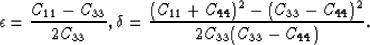$$\epsilon = \frac{C_{11}-C_{33}}{2C_{33}}, \delta = \frac{(C_{11}+C_{44})^2-(C_{33}-C_{44})^2}{2C_{33}(C_{33}-C_{44})}.$$ (2)

In deriving this dispersion relation it is assumed that the shear wave velocity is zero. This assumption holds for the remainder of this paper. Now for an elliptically anisotropic media we have $\eta = 0$ (in other words $\epsilon = \delta$) so that the above equation simplifies to:  

$$k_z = \sqrt{\frac{\omega^2}{v^2} - (k_x^2 + k_y^2) (1 + 2\epsilon)}.$$ (3)

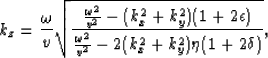
Thus in 3-D the vertical wavenumber for the full Double Square Root (DSR) form of the elliptically anisotropic migration operator is:  

$$k_z = \sqrt{\frac{\omega^2}{v(\bold s,z)^2} - (k_{sx}^2 + k_... ...a^2}{v(\bold r,z)^2} - (k_{rx}^2 + k_{ry}^2) (1 + 2\epsilon)} .$$ (4)

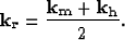
where $\bold{k_s}(k_{sx}, k_{sy})$ is the source wavenumber vector and $\bold{k_r}(k_{rx}, k_{ry})$ is receiver wavenumber vector. The equivalent form in midpoint-offset coordinates can be obtained by using the following simple transformations between the wavenumbers:  

$$\bold{k_s} = \frac{\bold{k_m} - \bold{k_h}}{2} ,$$ (5)

 

$$\bold{k_r} = \frac{\bold{k_m} + \bold{k_h}}{2} .$$ (6)

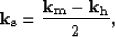
where $\bold{k_m}(k_{mx}, k_{my})$ is the midpoint wavenumber vector and $\bold{k_h}(k_{hx}, k_{hy})$ is the offset wavenumber vector. Substituting these transformations in equation (4) gives the vertical wavenumber for the elliptically anisotropic migration operator in midpoint-offset coordinates

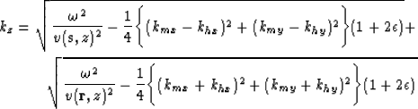$$\begin{eqnarray} k_z = \sqrt{\frac{\omega^2}{v(\bold s,z)^2} - \frac{1}{4}\Biggl... ...(k_{mx} + k_{hx})^2 + (k_{my} + k_{hy})^2\Biggr\} (1 + 2\epsilon)}\end{eqnarray}$$ (7)

The Common Azimuth downward continuation operator introduces a reduction in the dimensionality of the dataset by evaluating the new wavefield at a subsequent depth step only along the offset azimuth of the data in the previous depth step. The downward continuation operator Biondi and Palacharla (1996) can be expressed as:

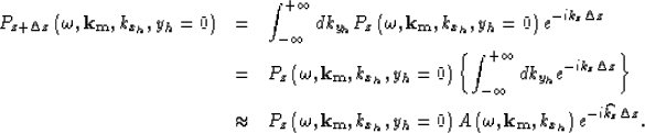$$\begin{eqnarray} P_{z+\Delta z} \left (\omega,{\bf k_m},k_{x_h},y_h=0 \right ) ... ...t (\omega,{\bf k_m},k_{x_h}\right ) e^{-i\widehat{k_z}\Delta z}.\end{eqnarray}$$ (8)

Since the common azimuth data is independent of k_hy, the integral can be pulled inside and analytically approximated by the stationary phase method. The stationary path approximation for the above operator can be found by setting the derivative of the wavenumber k_z with respect to k_hy to zero. This gives:  

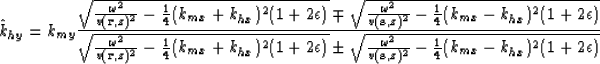$$\hat{k}_{hy} = k_{my}\frac{\sqrt{\frac{\omega^2}{v(\bold r,z... ...\bold s,z)^2} - \frac{1}{4}(k_{mx} - k_{hx})^2(1 + 2\epsilon)}}$$ (9)

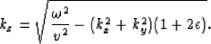
As in the case of the isotropic Common Azimuth migration operator, the above equation has two solutions. In choosing between these two solutions, we consider the limiting case of the in-line offset wavenumber (k_hx) equal to zero. In this case, one of the solution diverges while the other one, which has a minus sign on the numerator, goes to zero. We accept this solution. This gives the stationary path approximation for an elliptically anisotropic media. Hence, the new vertical wavenumber, $\hat{k_{ze}}$ for elliptically anisotropic media is evaluated along the stationary path given in equation(9) and is equal to:

$$\hat{k}_{ze} = DSR[\omega, \bold k_m, k_{hx}, \hat{k}_{hy},z ]$$ (10)