FEAVA effects in the image

Simple algebraic manipulations of Equation 1 show that in Angle-Domain Common Image Gathers (ADCIGs), for constant velocity and flat reflectors, the shape of the FEAVA path is given by  

$$z = z_a + \left\vert {m - m_a } \right\vert \cot \theta,$$ (2)

where z is depth, z_a is the depth of the heterogeneity, m is midpoint, m_a is the location of the anomaly, and $\theta$ is the reflection angle Vlad (2002). Figure plots this surface.

 

feavo_imag Figure 6 FEAVO path in ADCIGs, constant velocity, flat reflectors, heterogeneity 20m deep. Unlike in the data domain, the shape keeps on opening with depth and the arms of the ``V's'' are slightly curved.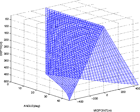

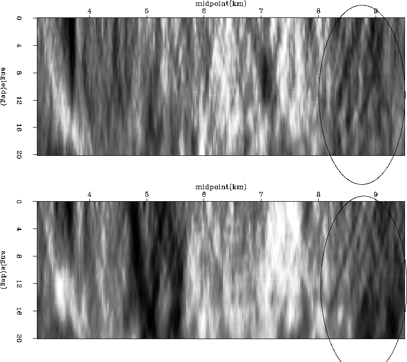
The ``Kjartansson V's'' are visible in the Grand Isle dataset after a v(z) survey-sinking migration. Figure shows two depth slices through the prestack image. The number of ``V''s is particularly large in this dataset, making it less than suitable for isolating and studying a FEAVO instantiation free from interference. In a less crowded area of the figure, the circled upside-down ``V'' shows vertical continuity as well as borders of polarity opposite from that of the main image, as predicted by finite-frequency wave theory Spetzler et al. (2004). Another property of data-domain FEAVO that gets carried over in the image domain is the dependence of the polarity of the effects on the sign of the velocity ``lenses'' (Figure ). The effects along the described paths have a finite width, as exemplified by Figure . In the case of velocity-caused FEAVO, the width of the path is linked to both the magnitude and the size of the heterogeneity. It is not known to what extent there is a magnitude-size ambiguity in the case of absorption. For both cases it may be possible to put an upper bound on the spatial extent of the anomaly based on the width of the FEAVO path, and this can be used as regularization in inversion for the anomalies or as an aid in interpretation.

Needed: A study of the link between the magnitude (intensity) and size (spatial extent) of the FEAVO source and the width of the FEAVA effects. This applies to data-domain effects too.

Migration removes any focusing effects which did not send energy outside the survey aperture Vlad (2005), so it will be easier to study FEAVA effects in the image than in the data - there is simply much less misplaced energy to interfere with the object of study. To properly view (and extract) FEAVA, one must first resolve the background velocity well enough that there is no residual first-order curvature in ADCIGs. FEAVA effects, being caused by anomalies much smaller than the cable length, will manifest themselves as slight traveltime wiggling accompanied by high/low amplitudes. Figure shows a synthetic example obtained of FEAVA effects ``in a pure state'', after all non-FEAVA energy has been removed.

The advantage of having less clutter in the image can be easily negated by a treatment of the data that emphasizes lack of noise over amplitude preservation. A comparation of Figure 2 in Vlad (2002) and Figure 6 in Vlad and Biondi (2002) shows an example of such an occurence. Using an amplitude-preserving processing and imaging flow is critical for correctly imaging the effects. Smearing the FEAVO effects with amplitude-careless processing is not removing them, but sweeping the dirt under the rug, since this will result in undesired FEAVO energy contaminating now unknown areas. Also, FEAVO removal may need to take into account the physics of the phenomenon, which need to be preserved. Vlad et al. (2003b) and Vlad and Tisserant (2004) describe the implementation of an amplitude-preserving shot-profile migration. The processing done before migration needs to use amplitude-preserving algorithms too.

Needed: A study of the amplitude properties of the offset-to-angle transformation used in creating the ADCIGs, and in particular the role of the regularization $\epsilon$, the variation of which has been observed to have significant results.

 

apslim
Figure 7 Depth slices 2.36km (top), 2.43km (bottom). Notice: (1) the slight opening of the upside-down, encircled ``V'' with depth, like in Figure ; (2) its opposite-polarity borders; and (3) the rectangular shaded areas spanning all angles which may denote ``legitimate'', reflector-caused AVO if reflectors are flat enough in this area.

An important point to note is that there is no relationship whatsoever between amplitude variations caused by focusing and those caused by variation of incidence angle on the reflector (FEAVO vs. ``legitimate'' AVO). The total amplitude of a reflector will show a superposition of the two effects, but the effects are physically independent from each other. FEAVO effects do not obey the sin<sup>2</sup> dependence between amplitude and reflection angle given by Shuey (1985). Figure offers an illustration of this property, and the ``FEAVO detection'' and ``FEAVO removal'' sections explore its the applications.