Methodology

We modify the flattening algorithm described in Lomask et al. (2005). The key regression is this overdetermined system:  

$$\boldsymbol{\nabla} \boldsymbol{\tau}\quad = \quad \bf p .$$ (1)

This equation means that we need to find a time-shift field $\boldsymbol{\tau}(x,y,z)$ such that its gradient approximates the dip $\bf{p}\rm (x,y,\boldsymbol{\tau})$. It is overdetermined because we are finding a single summed time shift field such that its two-dimensional gradient matches the dip in the x and y directions.

Imagine that after solving equation (1), the data residuals consist of spikes separated by relatively large distances. Then the estimated time shifts ${\boldsymbol \tau}$ would be piecewise smooth with jumps at the spike locations (fault locations), which is what we desire. However, in solving Equation (1), we use the least-squares criterion - minimization of the $\ell_2$ norm of the residual. Large spikes in the residual tend to be attenuated. In the model space, the solver smooths the time shifts across the spike location.

It is known that the $\ell_1$ norm is less sensitive to spikes in the residual Claerbout and Muir (1973); Darche (1989); Nichols (1994). Minimization of the $\ell_1$ norm makes the assumption that the residuals are exponentially distributed and have a ``long-tailed'' distribution relative to the Gaussian function assumed by the $\ell_2$ norm inversion.

 

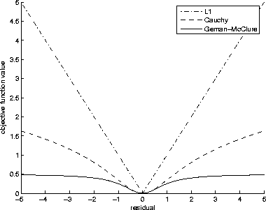
2 Figure 1 Comparison of the loss functions for the $\ell_1$, Cauchy, and Geman-McClure functions. Notice that the Geman-McClure is the most robust.

 

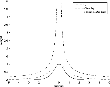
3 Figure 2 Comparison of weight functions for the $\ell_1$, Cauchy, and Geman-McClure functions. The Geman-McClure is most restrictive, this may be desirable for weighting faults.

Here, we compute non-linear model residual weights which force a Geman-McClure distribution, another long-tailed distribution which approximates an exponential distribution. A comparison of the loss functions for the $\ell_1$, Cauchy Claerbout (1999), and Geman-McClure functions is shown in Figure . Notice that the Geman-McClure is the most robust in that it is the least sensitive to outliers. Our weighted regression now is the following over-determined system:

$$\bf W^{j-1} \boldsymbol{\nabla} \boldsymbol{\tau}^j\quad = \bf W^{j-1} \bf p ,$$ (2)

where $\bf{ W^{j-1}}$ is the weight computed at the previous non-linear iteration.

Our method consists of recomputing the weights at each non-linear iteration, solving small piecewise Gauss-Newton linear problems. The IRLS algorithms converge if each minimization reaches a minimum for a constant weight. We perform the following non-linear iterations: starting with the weights ${\bf W^0}= \bf I$, at the j^th iteration the algorithm solves

		 iterate {    

$$\begin{eqnarray} \bf r \quad &=& \quad \bf W [\boldsymbol{\nabla} \boldsymbol{\t... ...} \quad &=& \quad \boldsymbol{\tau}_{k} + \Delta \boldsymbol{\tau}\end{eqnarray}$$ (3) (4) (5)

		  }    

At every non-linear iteration j^th iteration we re-estimate our Geman-McClure weight function:  

$$\bold W^{j-1} = \ {\bf diag} \left( {1\over{\left( {1+({\bf r}^{j-1})^2/\bar r^2}\right) ^2}} \right)$$ (6)

where $\bar r$ is an adjustable parameter. A comparison of weight functions for the $\ell_1$, Cauchy, and Geman-McClure functions is shown in Figure . Notice that the Geman-McClure creates the tightest, most precise weight. This should have the advantage of having a surgical-like effect of down-weighting spurious dips.