

Next: Chevron Gulf of Mexico
Up: examples of 3D flattening
Previous: examples of 3D flattening
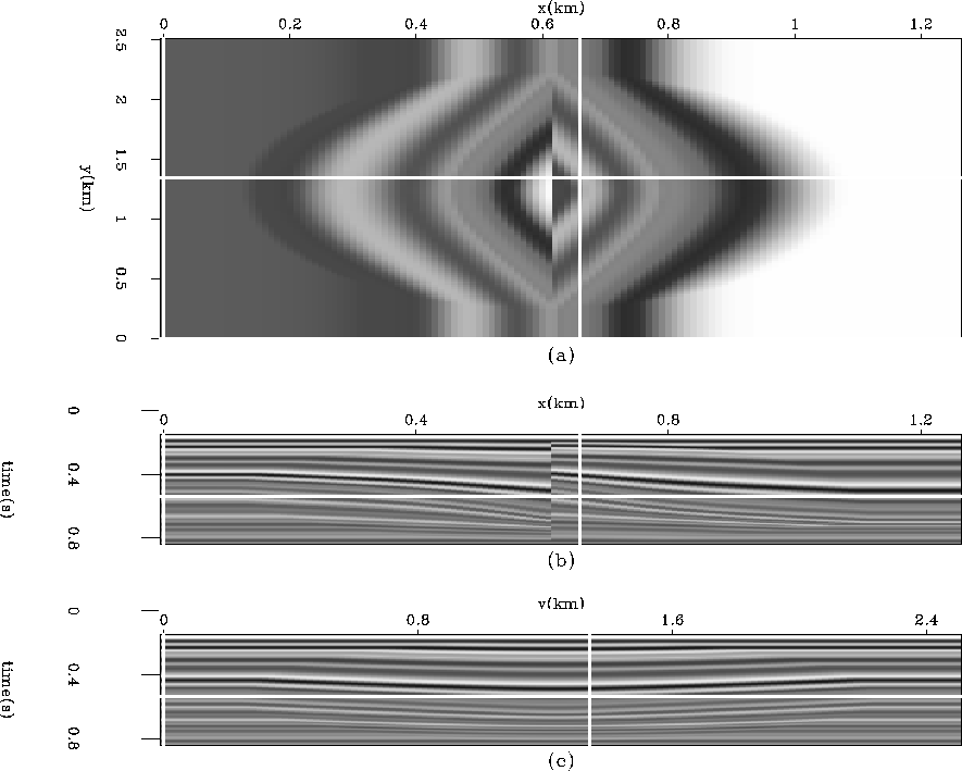
Figure ![[*]](http://sepwww.stanford.edu/latex2html/cross_ref_motif.gif) is a 3D synthetic dataset that presents two geological challenges. Firstly, the structure is changing with depth, requiring multiple non-linear iterations. Secondly, a significant fault is present in the middle of the cube. Dips estimated at fault discontinuities are, in general, inaccurate and will compromise the quality of the flattening result. However, knowing the position of the fault, we pass it as a weight to equation (12). In this case, we used a binary weight of 0's at the fault (and a few samples on each side) and 1's everywhere else.
is a 3D synthetic dataset that presents two geological challenges. Firstly, the structure is changing with depth, requiring multiple non-linear iterations. Secondly, a significant fault is present in the middle of the cube. Dips estimated at fault discontinuities are, in general, inaccurate and will compromise the quality of the flattening result. However, knowing the position of the fault, we pass it as a weight to equation (12). In this case, we used a binary weight of 0's at the fault (and a few samples on each side) and 1's everywhere else.
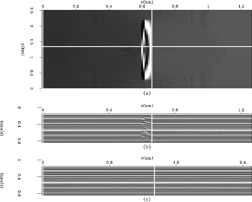
The flattening result is shown in Figure ![[*]](http://sepwww.stanford.edu/latex2html/cross_ref_motif.gif) . Notice the cube is very flat except in the area of the fault itself. This method is able to flatten this cube because we passed it a weight identifying the fault and the fault is limited laterally. That is, the tip-line of the fault is contained within the data cube, enabling dips to be summed around the fault.
. Notice the cube is very flat except in the area of the fault itself. This method is able to flatten this cube because we passed it a weight identifying the fault and the fault is limited laterally. That is, the tip-line of the fault is contained within the data cube, enabling dips to be summed around the fault.
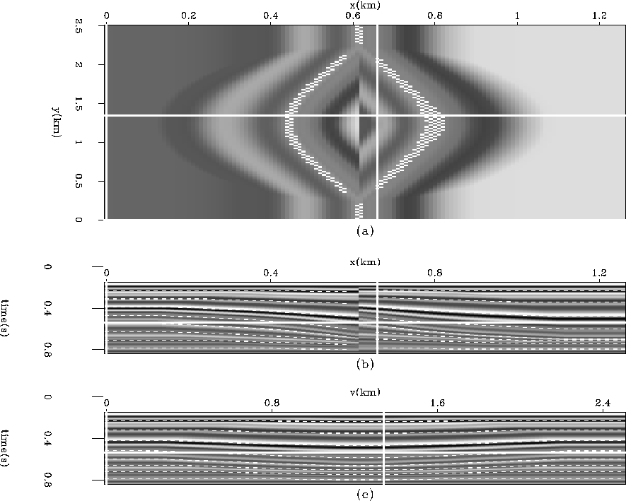
The estimated  field used to flatten data can also be used to reverse the process. That is, we can use the time-shifts to unflatten data that is already flat. By unflattening flat surfaces and overlaying them on the data, we are essentially picking any or all of the horizons in the data-cube. Figure
 ![[*]](http://sepwww.stanford.edu/latex2html/cross_ref_motif.gif) displays every 20th horizon overlain on the synthetic data shown in Figure
displays every 20th horizon overlain on the synthetic data shown in Figure ![[*]](http://sepwww.stanford.edu/latex2html/cross_ref_motif.gif) . We could just as easily have displayed every horizon but the image would appear too cluttered. Notice that the horizons are well tracked even across a fault.
. We could just as easily have displayed every horizon but the image would appear too cluttered. Notice that the horizons are well tracked even across a fault.
down_lap
Figure 1 A synthetic model with structure varying with depth that necessitates multiple iterations as well as a vertical discontinuity representing a fault. (a) The time slice at time= . (b) An in-line section at y=
 . (c) A cross-line section at x=
 .
.


 down_lap_flat
Figure 2 Result of flattening of Figure ![[*]](http://sepwww.stanford.edu/latex2html/cross_ref_motif.gif) . Notice it is flat on both sides of the fault zone. (a) The horizon
slice at time=
. Notice it is flat on both sides of the fault zone. (a) The horizon
slice at time= . (b) An in-line section at y=
 . (c) A cross-line section at x=
 .
.


 down_lap.horizon_overlay
Figure 3 Result of overlaying tracked horizons on the image in Figure ![[*]](http://sepwww.stanford.edu/latex2html/cross_ref_motif.gif) . The gap between reflections is where the weight was applied. It successfully tracks the horizons. (a) The time slice at time=
. The gap between reflections is where the weight was applied. It successfully tracks the horizons. (a) The time slice at time= . (b) An in-line section at y=
 . (c) A cross-line section at x=
 .
.


Next: Chevron Gulf of Mexico
Up: examples of 3D flattening
Previous: examples of 3D flattening
Stanford Exploration Project
5/3/2005
![[*]](http://sepwww.stanford.edu/latex2html/cross_ref_motif.gif) . Notice the cube is very flat except in the area of the fault itself. This method is able to flatten this cube because we passed it a weight identifying the fault and the fault is limited laterally. That is, the tip-line of the fault is contained within the data cube, enabling dips to be summed around the fault.
. Notice the cube is very flat except in the area of the fault itself. This method is able to flatten this cube because we passed it a weight identifying the fault and the fault is limited laterally. That is, the tip-line of the fault is contained within the data cube, enabling dips to be summed around the fault.


