$\omega$-$\mathbf{k}$ downward extrapolation

The previous section suggests an alternative implementation of mixed-domain migration. To see this more clearly, assume that, at each depth step, we downward continue the wavefield with the true velocities at that depth. In other words, compute $n_v=n_{\mathbf{x}}$ wavefields, each one corresponding to the model velocity at each spatial location. No split-step correction or higher-order approximation of k_z would then be required. The wavefield interpolation in $\omega$-$\mathbf{x}$ domain reduces to a simple selection of the appropriate wavefield, operation that can be expressed as:  

$$\mathbf{w}^{N+1}(j)=\sum_{l=1}^{n_v}\mathbf{w}_l^{N+1}(j)\delta_{lj}$$ (2)

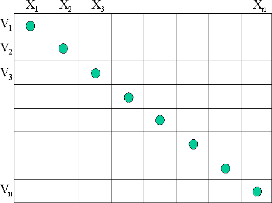
where $\mathbf{w}_l^{N+1}$ is the row of the array of wavefields extrapolated with the velocity V_l, and $\delta_{lj}$ is the Kronecker delta that selects from that row the corresponding j=l component. Notice that, since we are extrapolating as many wavefields as there are spatial positions (traces), $n_v=n_{\mathbf{x}}$. Figure  shows a schematic of the velocity selection.

 

bin_vels1 Figure 1 Diagram illustrating velocity selection when there are as many velocities as spatial locations.

In the $\omega$-$\mathbf{k}$ domain, Equation (2) becomes:  

$$\mathbf{W}^{N+1}=\sum_{l=1}^{n_v}\mathbf{W}_l^{N+1}\otimes e^{-ik_x\Delta x_l}$$ (3)

where $\Delta x_l=(l-1)\Delta x/n_x$ and we are using a single index to represent the spatial axis in order to simplify the notation. The symbol $\otimes$ represents circular convolution.

Notice that Equation (3) was derived without any approximation. Let's make the computations more explicit in order to gain a better appreciation for what it means:

$$\mathbf{W}^{N+1}(j)=\sum_{l=1}^{n_v}\sum_{m=\langle n_x\rangle} \mathbf{W}_l^{N+1}(m)e^{-ik_x(j-m)\Delta x_l}$$

where $\langle m\rangle$ means that the summation is over the range n_x with modulus n_x. That is,

$$\mathbf{W}^{N+1}(j)=\sum_{l=1}^{n_v}\sum_{m=1}^{n_x}\mathbf{W}^N(m)e^{-ik_{z_l}(m)\Delta z}e^{-ik_x(mod(j-m,n_x))\Delta x_l}.$$

Let $\tilde{m}_j=mod(j-m,n_x)$ and exchange the order of summation:

$$\mathbf{W}^{N+1}(j)=\sum_{m=1}^{n_x}\mathbf{W}^N(m)\sum_{l=1}^{n_v} e^{-i[k_{z_l}(m)\Delta z+k_x(\tilde{m}_j)]\Delta x_l}.$$

This equation shows that in order to compute the jth component of the extrapolated wavefield in the $\omega$-$\mathbf{k}$ domain, we need to take the dot product of the wavefield at the previous depth step with a vector that contains all the velocity and interpolation information. That is,  

$$\mathbf{W}^{N+1}(j)=\mathbf{W}^N\cdot \mathbf{f}_j$$ (4)

where $\mathbf{f}_j$ is the vector given by  

$$\mathbf{f}_j=\sum_{l=1}^{n_v}e^{-i[k_{z_l}(m)\Delta z+k_x(\tilde{m}_j)]\Delta x_l}.$$ (5)