Synthetic Test: Data Interpolation and Signal Extraction

In this section, we show the results of applying the sparse linear radon transform to synthetic teleseismic waveforms calculated with a velocity model (Figure ) from the LARSE-I experiment Baher et al. (2004). This model presents several real challenges in the form of large gradients in wavespeed found at the bottom of the Los Angeles basin, in the mid and the lower crust beneath the surface trace of the San Andreas, and at the base of the San Gabriel Mountains. After synthetic calculation, we extracted seismograms with actual station event geometries recorded during the experiment. This provides us a test dataset where we have prior knowledge of the crustal structure for assistance in identification of signal and noise phases and accurately sampled data for later comparison following interpolation.

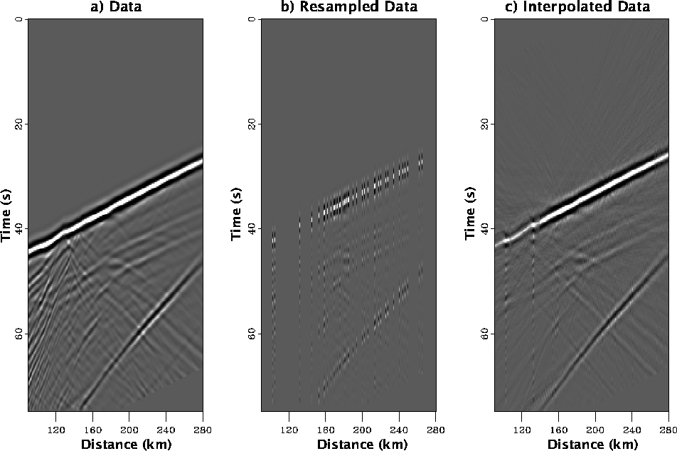
Figure shows the results of interpolation (c) of the resampled (b) data panel presented in (a) using the high resolution linear radon transform. The resampled synthetic data panel mimics the actual recording geometry used in the LARSE-I experiment and demonstrates the effect of wavefield aliasing due to irregular and coarse sampling. Despite the somewhat extreme spatial aliasing, the interpolated wavefield (c) contains many of the major features seen in (a) including the specularly scattered phases seen clearly between 200-240 km (see Figure for a more complete description), the high amplitude laterally coherent source wavefield, and the side reflection starting at 50 seconds at 280 km. In regions of especially sparse sampling, the amplitude of the interpolated data is slightly lower than in the original data panel and several butterfly artifacts can be identified. This suggests that finer, regular sampling would produce a more accurate and smooth data interpolation for many cases. Diffracted phases with large dips scattered from the basin bottom and the sharp Moho topography are severely aliased after resampling. For this example, we have applied a mute in the radon domain to regions outside of -0.18/0.05 s/km. This mute effectively removes surface scattered phases with large negative slopes and the side reflection with a positive slope near 0.1 s/km (Figure ).

 

SynthData-Result
Figure 4 Results of interpolation (c) of synthetic data (a) decimated to station spacing similar to that employed in the LARSE experiment (b). The decimated data panel shows how spatial aliasing can significantly hamper the ability to recover structure easily seen in the data in panel (a). Interpolation recovers many of the major planar arrivals especially in the regions with adequate sampling.

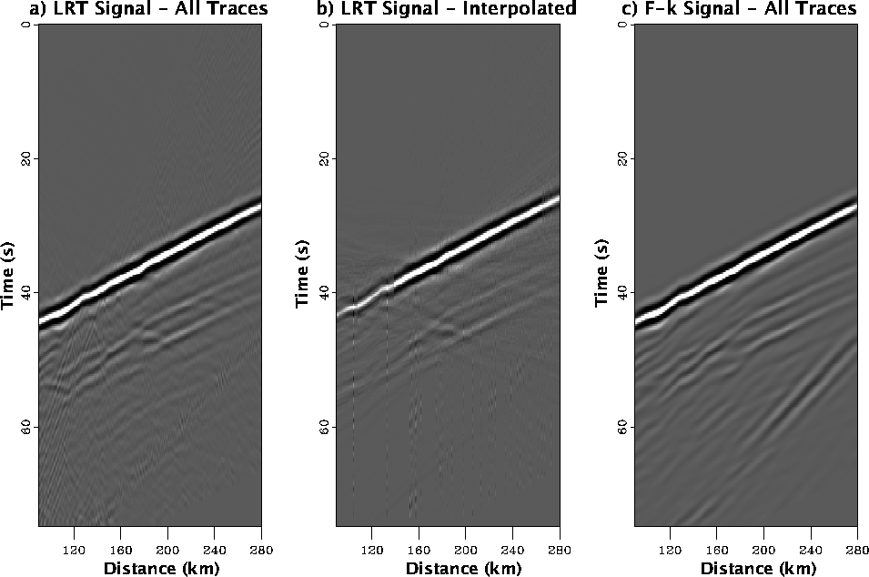
In Figure , we show the estimated signal from the synthetic data panel using both the linear radon transform (a and b) and standard f-k filtering (c). The comparison of the filtered signal using the interpolated traces (b) and all traces demonstrates how incomplete and irregular spatial sampling (e.g most teleseismic experiments) severely effects all procedures attempting to estimate and filter dips. Both the f-k and high resolution linear radon transform produce good results when the wavefield is adequately sampled. Unfortunately, this is rare and f-k methods do not offer an interpolation method except in cases of evenly spaced sampling. The filtered, interpolated data shown in panel (b) retains the medium to long wavelength, laterally coherent structures with similar moveout to the direct arrival. The majority of contamination from shallow scattering occurs in the region between 100-140 km. This is also the region of the poorest sampling and makes dip filtering very difficult. Therefore, some of what might be considered signal is lost in this area.

The linear radon transform excels in a few important areas of the data pnale when compared to the f-k filtered data panel. This is directly related to the suprerior dip and time resolution in the radon domain as compared to f-k space. For example, Moho diffraction tails seen between 160-180 km at $\sim$50 seconds are lost in the f-k section and remain in both radon filtered sections. Depending on the imaging algorithm chosen these diffraction tails could be considered signal or noise. A tighter mute in the radon domain could remove these features if necessary. This type of flexibility is not available with f-k filtering. Also, note the presence of the side reflection in the f-k filtered sections and its absence in the Radon filtered panels. Identification of the side reflection can occur in the f-k domain however separating without removing signal is difficult without using other attributes such as arrival time.

 

SynthSignal-Result
Figure 5 Comparison of signal panels calculated using the linear radon transform with all traces (a), linear radon transform with realistic station geometry (b), and f-k filtering using all traces. The results using the linear radon transform effectively muted the side reflection although this was not possible with f-k filtering without significantly degrading the signal. Diffraction tails from the complicated Moho topography between 160-200 km at 50 seconds have been removed by f-k filtering and replaced by artificial laterally continuous arrivals. The true character of these arrivals have not been modified by the radon algorithm although they could be removed with a modified mute window.

Possibly the easiest way to determine the effectiveness of the filtering operation is to look at what remains after subtracting the filtered section from the raw data (see Figure ). This provides a visual measure of what was removed and subsequently classified as noise. Figure shows the difference panels from high resolution radon filtering of all traces (a) and interpolated traces (b) and f-k filtering of all traces (c). The f-k panel was most effective with the near surface scattered energy although, the diffraction tails absent from the signal panel have reemerged here in the noise panel. Much of the major noise features are present on the noise estimates created with complete data panels (a and c). However, the interpolated data panel fails to identify a significant amount of energy from shallow features (near 40 s and between 100-140 km) as noise. Most likely this is because of dip ambiguities that result from coarse and irregular sampling. Ambiguous dips in a data panel are spread across a broader region in the radon domain and can not be completely muted.

 

SynthNoise-Result
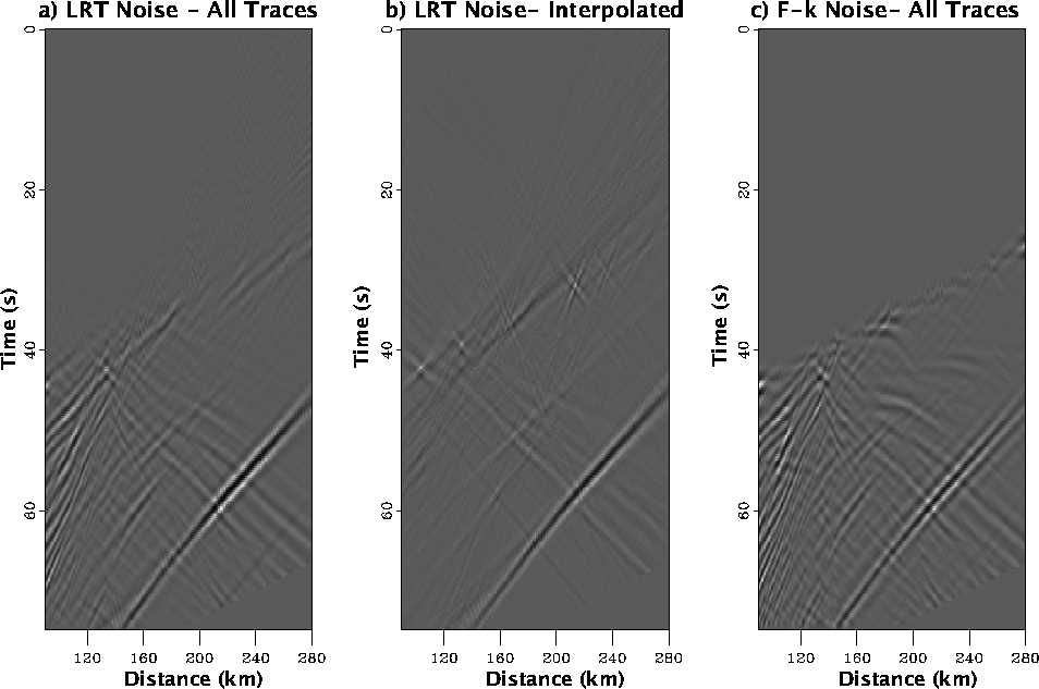Figure 6 Comparison of noise panels calculated by subtracting results shown in Figure from the original data panels shown in Figure . The truncated diffraction tails from the complicated Moho topography between 160-200 km at 50 seconds removed by f-k filtering have reappeared in the noise panels. The f-k filter was able to remove some of the energy from the side reflection (clearly seen in the noise panel) but this is still a significant arrival in Figure c. We prefer the noise estimation shown in (a) and (b) because we feel the character of the actual data and the noise have not been affected by spurious truncations and artifacts apparent in the f-k panels.