

Next: Noise separation in field
Up: Artman and Guitton: Combined
Previous: Theory
The first concern when solving inversion problems with over-complete
dictionaries is the potential for introduction of cross-talk
Claerbout (1992) into the model-space. A synthetic data
set was created to test the method to assure that this technique does
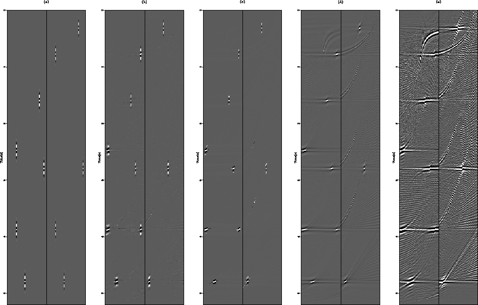
not allow this to happen. Figure ![[*]](http://sepwww.stanford.edu/latex2html/cross_ref_motif.gif) shows the inverted
models produced with the various methods compared to the least-squares
solution. The first panel is a bandlimited model from which data were
forward modeled, and the last four panels show the models produced by
the various inversion procedures.
shows the inverted
models produced with the various methods compared to the least-squares
solution. The first panel is a bandlimited model from which data were
forward modeled, and the last four panels show the models produced by
the various inversion procedures.
While the first two inversion schemes produce very
sparse model-spaces with no cross-talk, the l1 and l2 products
contain the familiar parabolas in the LRT domain due to data-space
hyperbolas and ellipses in the HRT domain from the linear events in
the data.
syn1
Figure 1 Synthetic model-space examples.
The model-space contains both radon domains. Thus, half way across
the slowness axis the plot changes from representing energy in the
hyperbolic radon domain to events in the linear radon domain. The
origin and sampling interval for both domains are the same in this
example. Panel (a) is the band-limited model. Panel (b) shows the BC
inversion result. Panel (c) shows the Cauchy result. Panel (d) shows the
l1 result. Panel (d) shows the l2 result.


The models produced by all the results are very good. The clip level
is deliberately set very low to bring out artifacts. While
the first two methods produce very sparse results, the l1 and l2
results contain sweeping artifacts and readily identifiable cross-talk
between the two model domains.
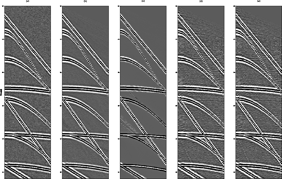
Figure ![[*]](http://sepwww.stanford.edu/latex2html/cross_ref_motif.gif) shows the forward modeled data from the models
produced from the various inversion techniques. The first panel is
the starting data. Once again, the clip
level has been set quite low to bring out the artifacts of the latter
inversion schemes. Amazingly, the two sparse inversion schemes,
especially the Cauchy inversion in panel (c), were able to remove much
of the 0.000001 variance noise added to the data. A small amount of
corrilary chatter can be seen in the Cauchy, l1, and l2 data
domains linear.
shows the forward modeled data from the models
produced from the various inversion techniques. The first panel is
the starting data. Once again, the clip
level has been set quite low to bring out the artifacts of the latter
inversion schemes. Amazingly, the two sparse inversion schemes,
especially the Cauchy inversion in panel (c), were able to remove much
of the 0.000001 variance noise added to the data. A small amount of
corrilary chatter can be seen in the Cauchy, l1, and l2 data
domains linear.
syn2
Figure 2 Forward modeled data from the
inversion results presented in Figure ![[*]](http://sepwww.stanford.edu/latex2html/cross_ref_motif.gif) . Panel (a) is
the band-limited model. Panel (b) shows the BC inversion result.
Panel (c) shows the Cauchy result. Panel (d) shows the l1
result. Panel (d) shows the l2 result.
. Panel (a) is
the band-limited model. Panel (b) shows the BC inversion result.
Panel (c) shows the Cauchy result. Panel (d) shows the l1
result. Panel (d) shows the l2 result.


The inversion schemes designed for sparse model domains have produced
models with no cross-talk between the two operators. The l1 and
l2 inversions have allowed the transmission of energy between the
two domains. However, the forward modeled data from all the methods
show more than adequate results with only minor noise introduced in
the immediate vicinity of the various events. Importantly, even the
very steeply dipping events are well modeled despite being severely
aliased. It should be noted however, that the first two schemes will
not produce satisfactory data-space results given realistic
split-spread gathers. Their short-comings are from linear events that
do not continue completely across the entire data domain. The sparse
model domains do not have sufficient freedom to add fictitious model
energy to cancel events that do not exactly eminate from the origin of
the shot (ie. exit the gather at t=0, x=0). Throughout this
effort, only off-end gathers will be used.


Next: Noise separation in field
Up: Artman and Guitton: Combined
Previous: Theory
Stanford Exploration Project
5/3/2005
![[*]](http://sepwww.stanford.edu/latex2html/cross_ref_motif.gif) shows the inverted
models produced with the various methods compared to the least-squares
solution. The first panel is a bandlimited model from which data were
forward modeled, and the last four panels show the models produced by
the various inversion procedures.
shows the inverted
models produced with the various methods compared to the least-squares
solution. The first panel is a bandlimited model from which data were
forward modeled, and the last four panels show the models produced by
the various inversion procedures.

