PEFs in the data space

Once we attempt to interpolate this dataset using only the sparse tracks, the above method no longer works, as no region would have enough contiguous data on which to estimate a PEF. In this case we will pay more attention to how our data are spatially distributed. The known data points in the model space are distributed along curved crossing tracks, making it very difficult to estimate a PEF in this space, as shown in Figure . However, in the data space of the fitting goals (1) of the previous section, the data are sampled in a regular space: a series of regularly-sampled tracks, as shown in Figures and .

 

sptracks
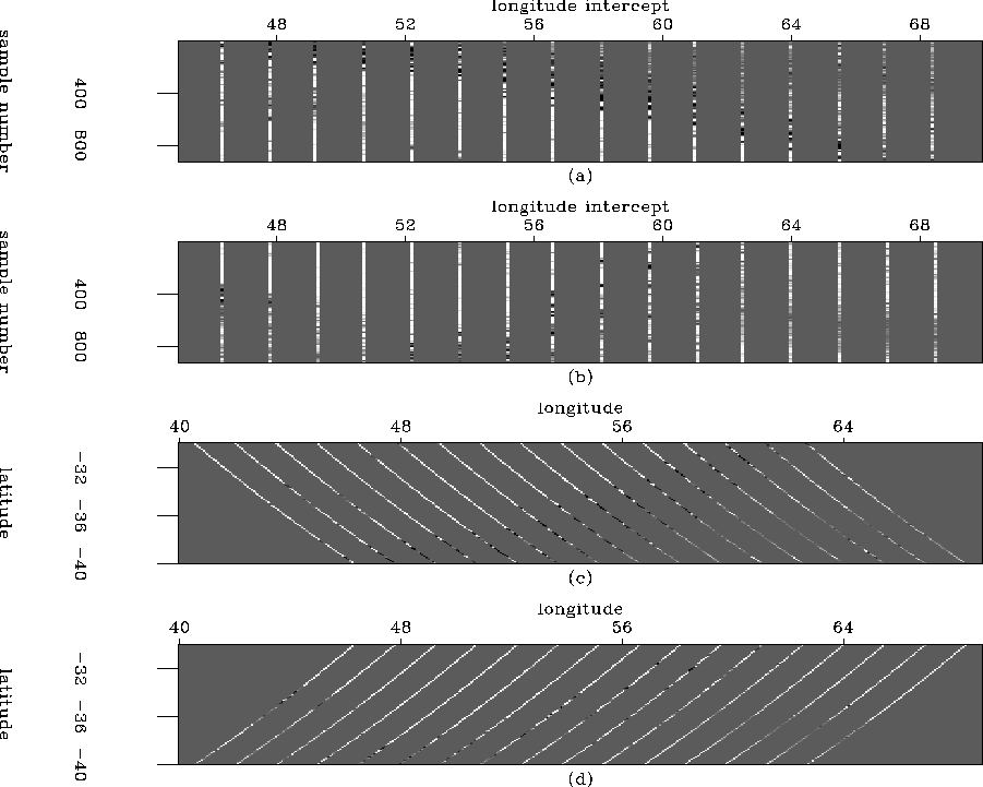
Figure 3 Sparse tracks, (a) ascending and (b) descending in model space, and (c) ascending and (d) descending tracks in data space.

 

detracks
Figure 4 Dense tracks, (a) ascending and (b) descending in model space, and (c) ascending and (d) descending tracks in data space.

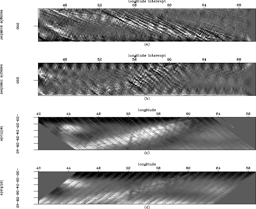
Since these data are collected in two series of one-dimensional tracks, it would be easiest to estimate a pair of one-dimensional PEFs on these two sets of tracks, as shown in the top halfs of Figures and .

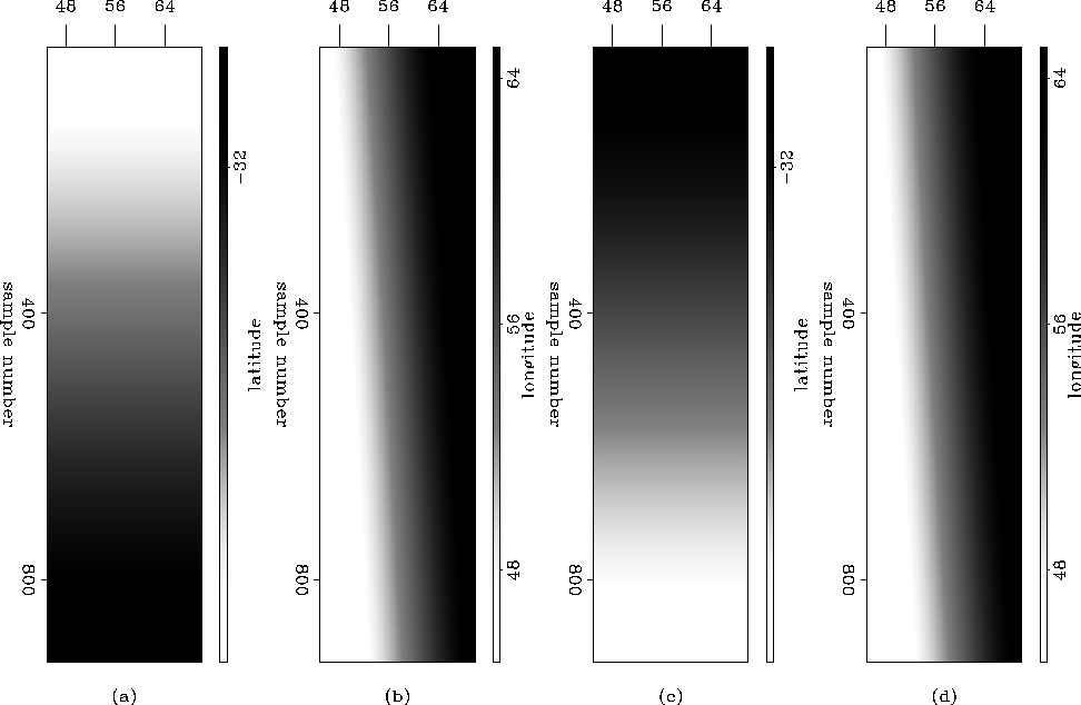
We now have two PEFs which have been estimated in a data space, but the model which we wish to regularize with these PEFs is in a different space. This requires the introduction of two additional linear interpolation operators ${\bf L_1}$ and ${\bf L_2}$, which pull bins from the model space into the ascending and descending track data spaces, respectively. The mappings used for these operators are shown in Figure .

 

maps
Figure 5 Mappings from data space to model space, all shown in data space. From the top down: ascending tracks latitude, ascending tracks longitude, descending tracks latitude, descending tracks longitude.

Now that we have both two prediction-error filters for regularizations operators as well as linear interpolation operators that pull model points into the data space, we can put everthing together in the following fitting goals,

$$\begin{eqnarray} \ {\bf W} \frac{d}{dt}[{\bf L}{\bf m} -{\bf d}] &\approx& {\bf ... ...ld 0 \nonumber \\ \epsilon \bold{A_{2}L_{2}m} &\approx& \bold 0, \end{eqnarray}$$ (3)

where L pulls model points (m) to where we have data (d), $\bold{A_{1}}$ and $\bold{A_{2}}$ are 1D PEFs that are estimated on the ascending and descending tracks in the data space, respectively, and $\bold{L_{1}}$ and $\bold{L_{2}}$ are linear interpolation operators that pull model points into the ascending and descending track data spaces, respectively. $\epsilon$ is a tradeoff parameter between the data fitting and model styling goals.

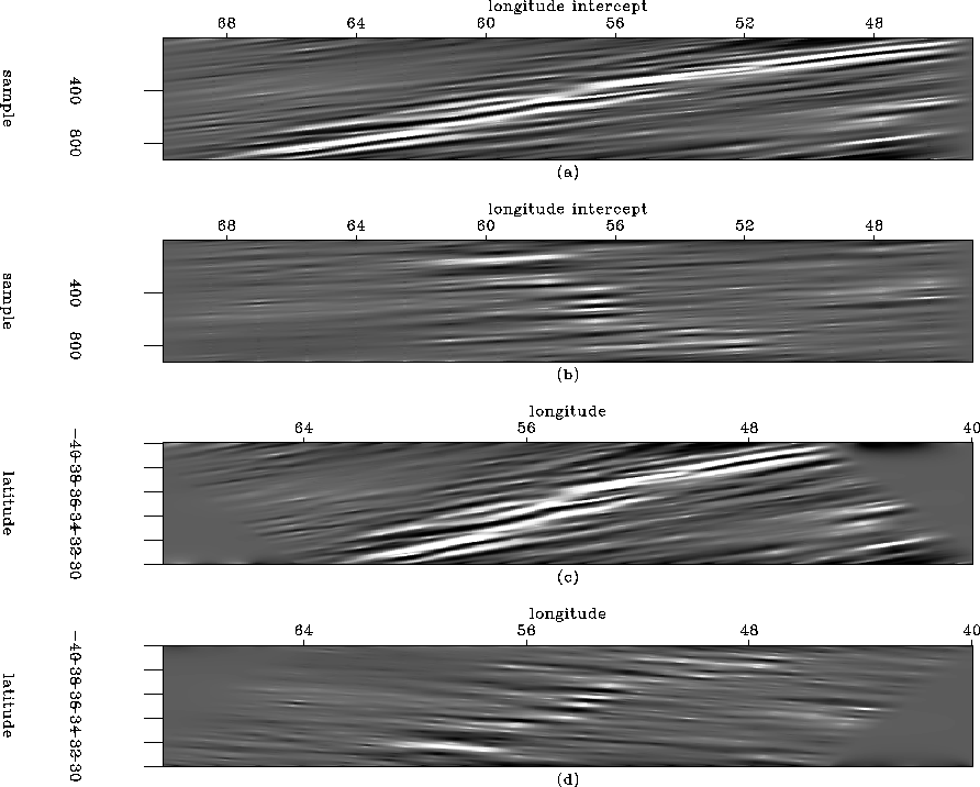
The 1D PEFs can also be replaced by 2D PEFs that are estimated by scaling the filter so that it covers multiple sparse tracks. If this approach is taken, the interpolation can occur in the data space where the PEFs are estimated (using a single PEF for each of the two track spaces), or in the model space (using both PEFs simultaneously). The more straightforward data-space interpolation is shown in Figure .

 

dataspinterp
Figure 6 Interpolation of the two different track spaces (a) and (b). (c) and (d) contain the same results mapped into model space. The correct strike of the ridge is identified by the ascending tracks but not the descending tracks.

Figures a and b are simply the interpolation of the data space with 2D PEFs estimated on the sparse tracks. Figures c and d are those interpolated results mapped back to the model space by using fitting goals (1), where the input data are now the interpolated sets of tracks in the first two panels. Since fitting goals (1) were applied when generating the new tracks, the track derivative is no longer necessary.

The results are mixed, as Figure c shows that the trend of the ridge was correctly identified by the PEF estimated on the ascending tracks. The PEF estimated on the descending tracks did not fare so well, as the direction of the ridge in the interpolated tracks of Figure d does not match the densely sampled tracks in Figure d. This is because the descending tracks are oblique to the structure, so the structure is aliased beyond the point where a spaced PEF can interpolate accurately. In either case, the result is better than that obtained with a Laplacian, and in the case of the ascending tracks is not that far from the PEF estiamted on a fully-sampled model space shown in Figure c.