

Next: conclusion
Up: Guitton et al.: Non-linear
Previous: 2-D data examples
The 3-D algorithm is tested on two datasets from the Gulf of Mexico.
Figures ![[*]](http://sepwww.stanford.edu/latex2html/cross_ref_motif.gif) a,
a, ![[*]](http://sepwww.stanford.edu/latex2html/cross_ref_motif.gif) b,
and
b,
and ![[*]](http://sepwww.stanford.edu/latex2html/cross_ref_motif.gif) c show the input data, the picked
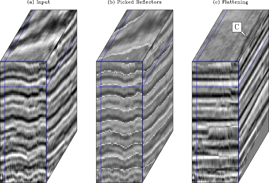
reflector, and the flattening result for the first dataset. The size
of this dataset is 100x100x100 samples. After flattening in Figure
c show the input data, the picked
reflector, and the flattening result for the first dataset. The size
of this dataset is 100x100x100 samples. After flattening in Figure
![[*]](http://sepwww.stanford.edu/latex2html/cross_ref_motif.gif) c, a channel is now clearly visible.
Note that the picked reflectors in Figure
c, a channel is now clearly visible.
Note that the picked reflectors in Figure
![[*]](http://sepwww.stanford.edu/latex2html/cross_ref_motif.gif) b follow extremely well the true
reflectors. Again, this result is obtained at no cost and is readily
available from the estimation of
b follow extremely well the true
reflectors. Again, this result is obtained at no cost and is readily
available from the estimation of  .
.
Figures ![[*]](http://sepwww.stanford.edu/latex2html/cross_ref_motif.gif) a,
a, ![[*]](http://sepwww.stanford.edu/latex2html/cross_ref_motif.gif) b,
and
b,
and ![[*]](http://sepwww.stanford.edu/latex2html/cross_ref_motif.gif) c show the input data, the picked
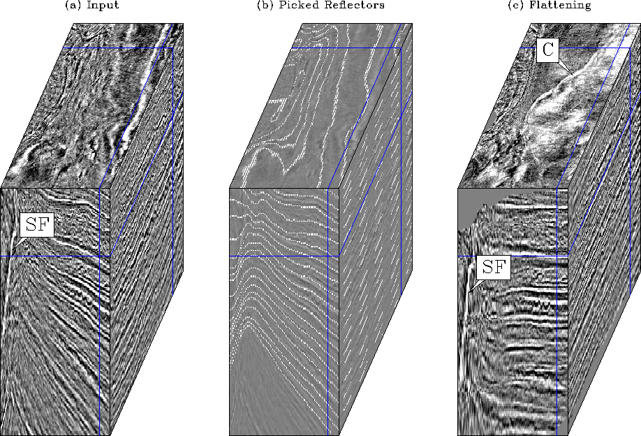
reflector, and the flattening result for the second dataset.
The size of this dataset is 200x200x200 samples.
It features more complicated structures such as a large
salt body on the left (shown as SF) and faults. Nothing was done to
pick the faults, as suggested by Lomask et al. (2005). Nevertheless,
the flattening result in Figure
c show the input data, the picked
reflector, and the flattening result for the second dataset.
The size of this dataset is 200x200x200 samples.
It features more complicated structures such as a large
salt body on the left (shown as SF) and faults. Nothing was done to
pick the faults, as suggested by Lomask et al. (2005). Nevertheless,
the flattening result in Figure ![[*]](http://sepwww.stanford.edu/latex2html/cross_ref_motif.gif) c
highlights one channel on the depth slice that was not previously visible.
The picking result in Figure
c
highlights one channel on the depth slice that was not previously visible.
The picking result in Figure ![[*]](http://sepwww.stanford.edu/latex2html/cross_ref_motif.gif) b is also
very accurate.
b is also
very accurate.
3D-data-shoal-test
Figure 7 (a) Model. (b)
Automatic picking of few horizons. (c) Flattening result.
The picked horizons follow extremely well the structure of the data.
On the time slice (top panel) a channel (marked as C), previously unseen in
the data, is revealed by the flattening process.


 3D-ExxonMobil-data
Figure 8 (a) Model. (b)
Automatic picking of few horizons. (c) Flattening result.
On the depth slice (top panel) a channel (marked as C), previously unseen in
the data, is revealed by the flattening process. Arrow SF shows the
salt flanks.


Next: conclusion
Up: Guitton et al.: Non-linear
Previous: 2-D data examples
Stanford Exploration Project
5/3/2005
![[*]](http://sepwww.stanford.edu/latex2html/cross_ref_motif.gif) a,
a, ![[*]](http://sepwww.stanford.edu/latex2html/cross_ref_motif.gif) b,
and
b,
and ![[*]](http://sepwww.stanford.edu/latex2html/cross_ref_motif.gif) c show the input data, the picked
reflector, and the flattening result for the second dataset.
The size of this dataset is 200x200x200 samples.
It features more complicated structures such as a large
salt body on the left (shown as SF) and faults. Nothing was done to
pick the faults, as suggested by Lomask et al. (2005). Nevertheless,
the flattening result in Figure
c show the input data, the picked
reflector, and the flattening result for the second dataset.
The size of this dataset is 200x200x200 samples.
It features more complicated structures such as a large
salt body on the left (shown as SF) and faults. Nothing was done to
pick the faults, as suggested by Lomask et al. (2005). Nevertheless,
the flattening result in Figure ![[*]](http://sepwww.stanford.edu/latex2html/cross_ref_motif.gif) c
highlights one channel on the depth slice that was not previously visible.
The picking result in Figure
c
highlights one channel on the depth slice that was not previously visible.
The picking result in Figure ![[*]](http://sepwww.stanford.edu/latex2html/cross_ref_motif.gif) b is also
very accurate.
b is also
very accurate.

