2-D data examples

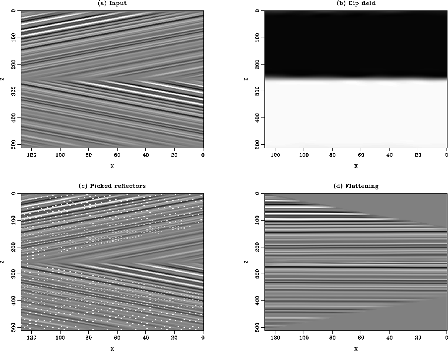
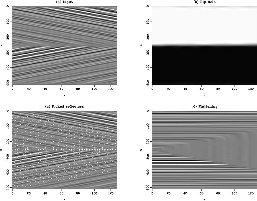
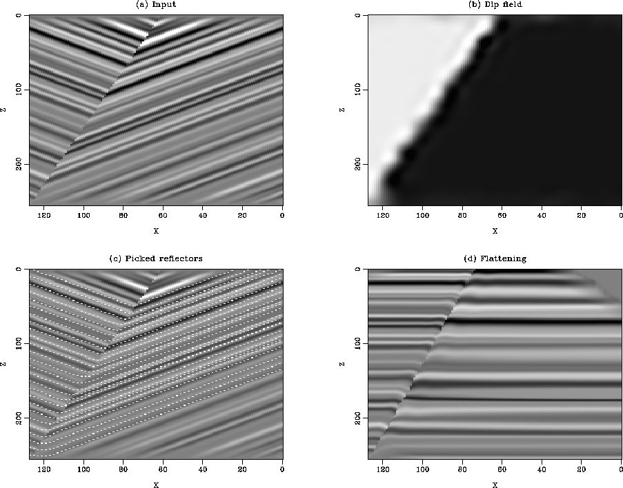
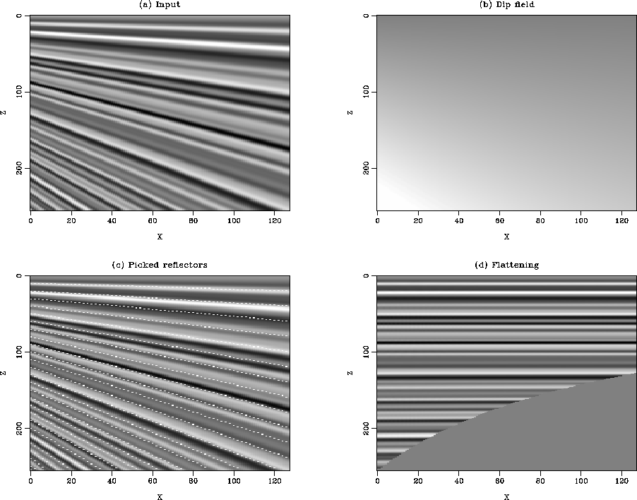
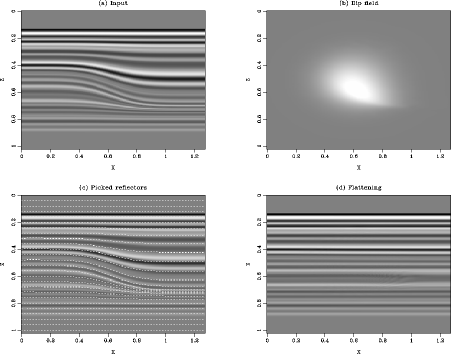
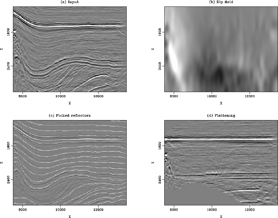
The 2-D algorithm, a simple extension of the 3-D algorithm, is illustrated first on five synthetic (Figures to ) and one field data examples (Figure ). All these figures are organized as follows: panel (a) shows the input data, panel (b) shows the estimated dip field using Fomel's technique Fomel (2002), (d) shows the picking result where the seed point starts from the reference trace every ten samples in time/depth, and (d) shows the flattening result. The field data example is a 2-D slice extracted from the Elf (now Total) L7D dataset after common-azimuth depth migration Vaillant et al. (2000). All these examples illustrate that the time/depth delay estimation process is very accurate and robust.

 

unconformity
Figure 1 (a) Model. (b) Estimated dips. (c) Automatic picking of few horizons. (d) Flattening result. The first trace is used for reference.

 

unconformity2
Figure 2 (a) Model. (b) Estimated dips. (c) Automatic picking of few horizons. (d) Flattening result. The first trace is used for reference.

 

unconformity3
Figure 3 (a) Model. (b) Estimated dips. (c) Automatic picking of few horizons. (d) Flattening result. The smoothness of the estimated dips introduce small errors in the flattening result. The first trace is used for reference.

 

thinning3
Figure 4 (a) Model. (b) Estimated dips. (c) Automatic picking of few horizons. (d) Flattening result. The first trace is used for reference.

 

down_lap2D
Figure 5 (a) Model. (b) Estimated dips. (c) Automatic picking of few horizons. (d) Flattening result. The first trace is used for reference.

 

elf2D
Figure 6 (a) Model. (b) Estimated dips. (c) Automatic picking of few horizons. (d) Flattening result. The picked horizons follow extremely well the structure of the data. The trace at X=12000 is used for reference.