Explicitly computing the Hessian is possible when following a target-oriented strategy that exploits the Hessian sparsity and structure. We created a synthetic dataset, using equation 6, with a constant-reflectivity flat reflector (at ![]() ) in a constant-velocity medium (
) in a constant-velocity medium (![]() ).
Assuming a land acquisition geometry, where the shots and receivers were positioned every
).
Assuming a land acquisition geometry, where the shots and receivers were positioned every ![]() on the interval
on the interval ![]() . Valenciano and Biondi (2004) discuss in detail the banded nature and sparsity of the Hessian matrix for the constant-velocity model.
. Valenciano and Biondi (2004) discuss in detail the banded nature and sparsity of the Hessian matrix for the constant-velocity model.
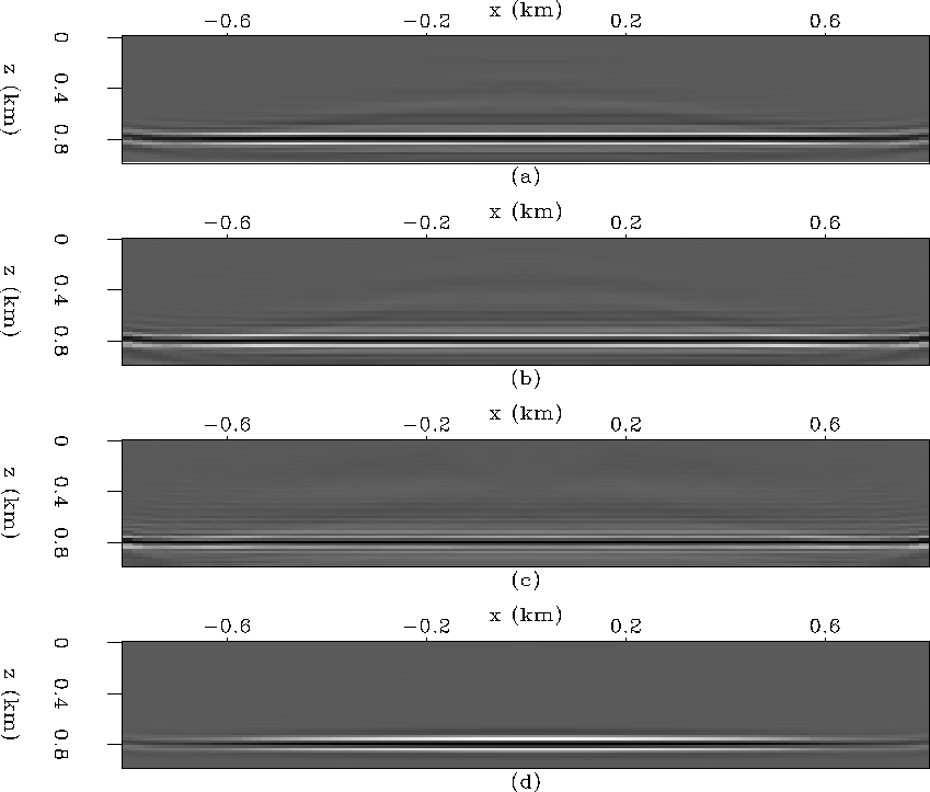
Figure ![[*]](http://sepwww.stanford.edu/latex2html/cross_ref_motif.gif) shows a
shows a ![]() coefficient filter at constant depth as the x coordinate moves from the corner to the center of the acquisition. Figure
coefficient filter at constant depth as the x coordinate moves from the corner to the center of the acquisition. Figure ![[*]](http://sepwww.stanford.edu/latex2html/cross_ref_motif.gif) a shows point 1, with coordinates
a shows point 1, with coordinates ![]() (corner of the acquisition). Figure
(corner of the acquisition). Figure ![[*]](http://sepwww.stanford.edu/latex2html/cross_ref_motif.gif) b shows point 2, with coordinates
b shows point 2, with coordinates ![]() . Figure
. Figure ![[*]](http://sepwww.stanford.edu/latex2html/cross_ref_motif.gif) c shows point 3, with coordinates
c shows point 3, with coordinates ![]() . Figure
. Figure ![[*]](http://sepwww.stanford.edu/latex2html/cross_ref_motif.gif) d shows point 4, with coordinates
d shows point 4, with coordinates ![]() (at the center of the acquisition).
(at the center of the acquisition).
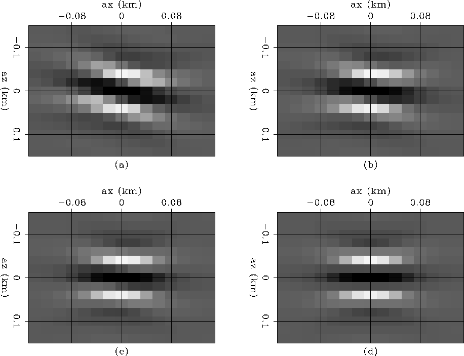 |
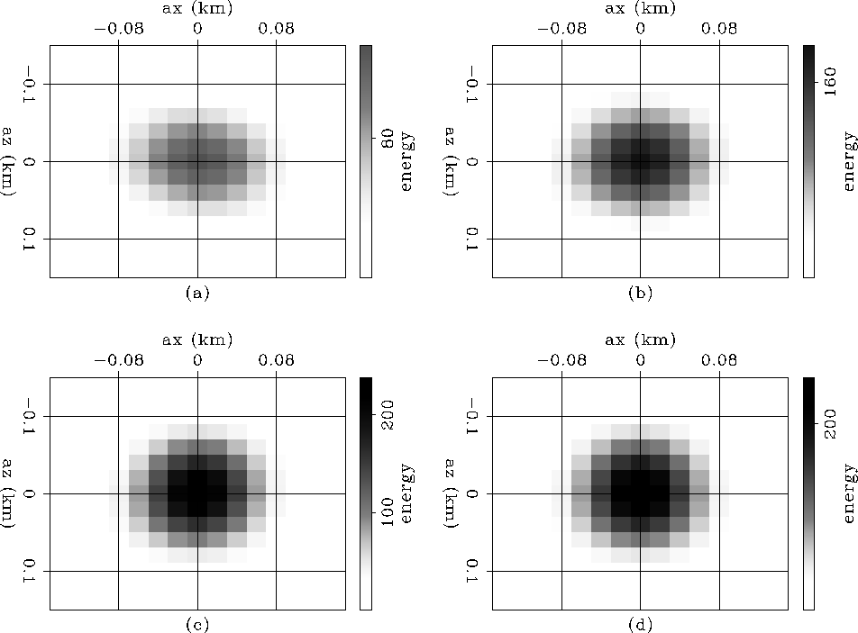
Figure ![[*]](http://sepwww.stanford.edu/latex2html/cross_ref_motif.gif) shows the envelope of the
shows the envelope of the ![]() coefficient filter shown in Figure
coefficient filter shown in Figure ![[*]](http://sepwww.stanford.edu/latex2html/cross_ref_motif.gif) . The energy of the ellipses become dimer away from the center, indicating that these points have lower illumination due to the acquisition geometry. To correct this effect we computed the least-squares inverse image, by the method described in the above section.
. The energy of the ellipses become dimer away from the center, indicating that these points have lower illumination due to the acquisition geometry. To correct this effect we computed the least-squares inverse image, by the method described in the above section.
 |
Two different numbers of filter coefficients were used. Figures ![[*]](http://sepwww.stanford.edu/latex2html/cross_ref_motif.gif) and
and ![[*]](http://sepwww.stanford.edu/latex2html/cross_ref_motif.gif) show the inversion results for a filter of
show the inversion results for a filter of ![]() coefficients, whereas Figures
coefficients, whereas Figures ![[*]](http://sepwww.stanford.edu/latex2html/cross_ref_motif.gif) and
and ![[*]](http://sepwww.stanford.edu/latex2html/cross_ref_motif.gif) show the inversion results for a filter of
show the inversion results for a filter of ![]() coefficients. Figure
coefficients. Figure ![[*]](http://sepwww.stanford.edu/latex2html/cross_ref_motif.gif) shows a comparison of the best results of both filter sizes.
shows a comparison of the best results of both filter sizes.
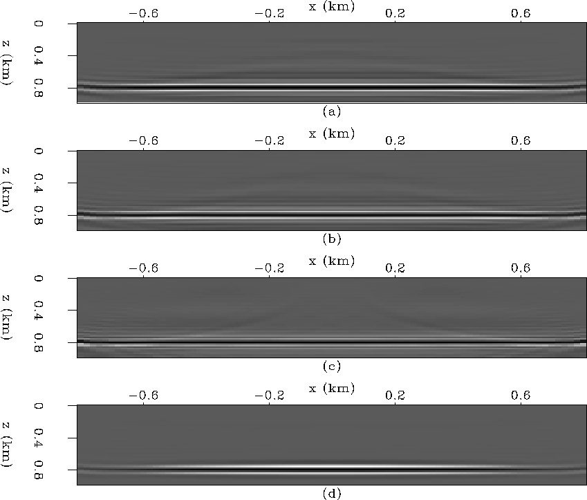
The panels in Figure ![[*]](http://sepwww.stanford.edu/latex2html/cross_ref_motif.gif) show the least-squares inverse image for different numbers of iterations for a filter of
show the least-squares inverse image for different numbers of iterations for a filter of ![]() coefficients:
coefficients: ![[*]](http://sepwww.stanford.edu/latex2html/cross_ref_motif.gif) a for 10 iterations,
a for 10 iterations, ![[*]](http://sepwww.stanford.edu/latex2html/cross_ref_motif.gif) b for 20 iterations,
b for 20 iterations, ![[*]](http://sepwww.stanford.edu/latex2html/cross_ref_motif.gif) c for 100 iterations, and
c for 100 iterations, and ![[*]](http://sepwww.stanford.edu/latex2html/cross_ref_motif.gif) d for migration. Notice how the image amplitudes become more even.
Figure
d for migration. Notice how the image amplitudes become more even.
Figure ![[*]](http://sepwww.stanford.edu/latex2html/cross_ref_motif.gif) shows the comparison of the same least-squares inverse image results at the reflector depth. The image amplitude after 100 iterations is the best result. The conjugate gradient algorithm further balances the image amplitudes, which reduces the effects of the acquisition geometry and the bandlimited characteristic of the seismic data.
shows the comparison of the same least-squares inverse image results at the reflector depth. The image amplitude after 100 iterations is the best result. The conjugate gradient algorithm further balances the image amplitudes, which reduces the effects of the acquisition geometry and the bandlimited characteristic of the seismic data.
 |
|
inv_const_pp_11
Figure 4 Amplitudes extracted at reflector depth from Figure ![[*]](http://sepwww.stanford.edu/latex2html/cross_ref_motif.gif) , filter size of , filter size of | 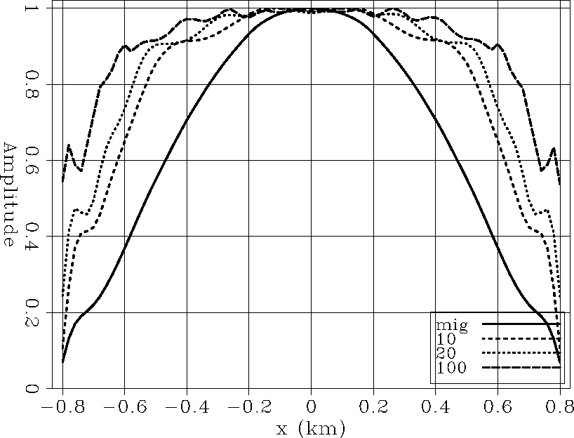 |
The panels in Figure ![[*]](http://sepwww.stanford.edu/latex2html/cross_ref_motif.gif) show the least-squares inverse image for different number of iterations for a filter of
show the least-squares inverse image for different number of iterations for a filter of ![]() coefficients:
coefficients: ![[*]](http://sepwww.stanford.edu/latex2html/cross_ref_motif.gif) a for 10 iterations,
a for 10 iterations, ![[*]](http://sepwww.stanford.edu/latex2html/cross_ref_motif.gif) b for 20 iterations,
b for 20 iterations, ![[*]](http://sepwww.stanford.edu/latex2html/cross_ref_motif.gif) c for 100 iterations, and
c for 100 iterations, and ![[*]](http://sepwww.stanford.edu/latex2html/cross_ref_motif.gif) d for migration. Notice again, how the image amplitudes become more even.
Figure
d for migration. Notice again, how the image amplitudes become more even.
Figure ![[*]](http://sepwww.stanford.edu/latex2html/cross_ref_motif.gif) shows the comparison of the same least-squares inverse image results at the reflector depth. The image amplitude after 100 iterations is the best result. The conjugate gradient algorithm once again further balances the image amplitudes.
shows the comparison of the same least-squares inverse image results at the reflector depth. The image amplitude after 100 iterations is the best result. The conjugate gradient algorithm once again further balances the image amplitudes.
 |
|
inv_const_pp_15
Figure 6 Amplitudes extracted at reflector depth from Figure ![[*]](http://sepwww.stanford.edu/latex2html/cross_ref_motif.gif) , filter size of , filter size of | 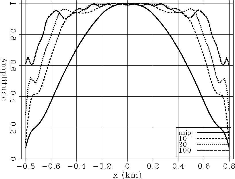 |
Figure ![[*]](http://sepwww.stanford.edu/latex2html/cross_ref_motif.gif) compares the migration result to the best inversion results for filter sizes
compares the migration result to the best inversion results for filter sizes ![]() coefficients,
coefficients, ![]() coefficients. There is not much difference in the recovered amplitudes, thus a filter size of
coefficients. There is not much difference in the recovered amplitudes, thus a filter size of ![]() should be sufficient.
should be sufficient.
|
inv_const_filter
Figure 7 Comparison the migration result to the best inversion results for filter sizes | 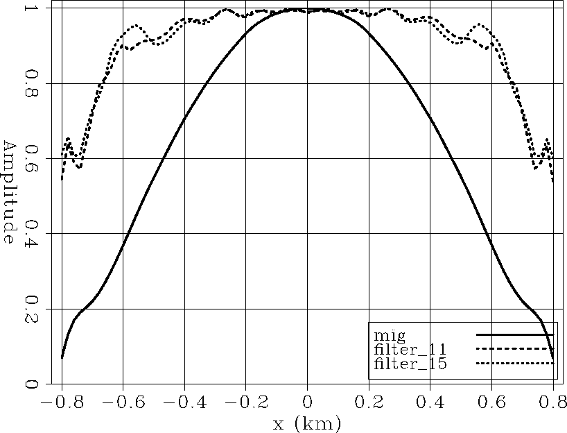 |