Fréchet derivative integral kernels

Consider a (nonlinear) function $\bf{f}$ mapping one element of the functional model space $\mod$ to one element of the functional data space $\dat$: 

$$\dat = \bf{f}\lp \mod \rp \;.$$ (70)

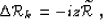
The tangent linear application to $\bf{f}$ at point $\mod=\mod_0$ is a linear operator ${\bf F}_0$ defined by the expansion  

$$\bf{f}\lp \mod_0+\delta \mod\rp = \bf{f}\lp \mod_0\rp + {\bf F}_0\delta \mod+ \dots \;,$$ (71)

where $\delta \mod$ is a small perturbation in the model space. The tangent linear application ${\bf F}_0$ is also known under the name of Fréchet derivative of $\bf{f}$ at point $\mod_0$ (109).

 

fat3.sC
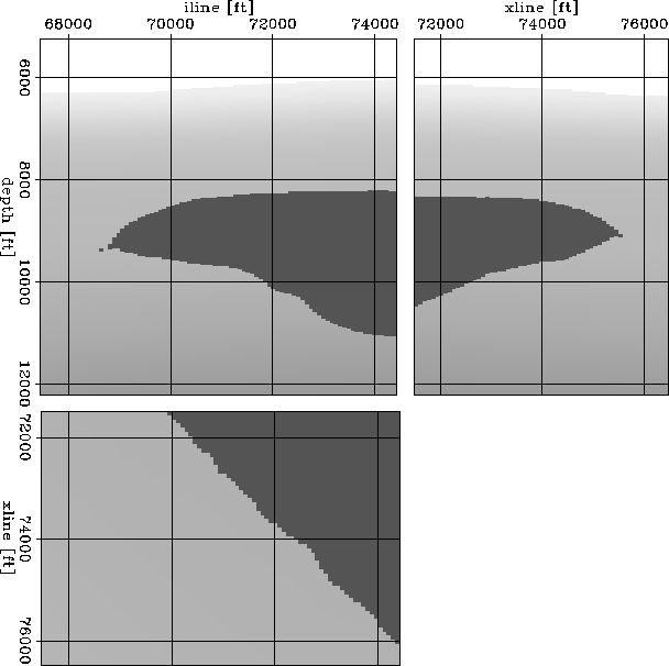
Figure 12 3D slowness model.

 

fat3.fp3
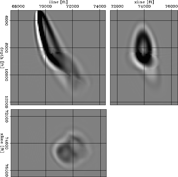
Figure 13 3D sensitivity kernels for wave-equation MVA. The frequency range is 1-16 Hz. The kernels are complicated by the multipathing occurring as waves propagate through the rough salt body. The image perturbation corresponds to a kinematic shift.

 

fat3.fq3
Figure 14 3D sensitivity kernels for wave-equation MVA. The frequency range is 1-16 Hz. The kernels are complicated by the multipathing occurring as waves propagate through the rough salt body. The image perturbation corresponds to an amplitude scaling.

 

fat3.svty
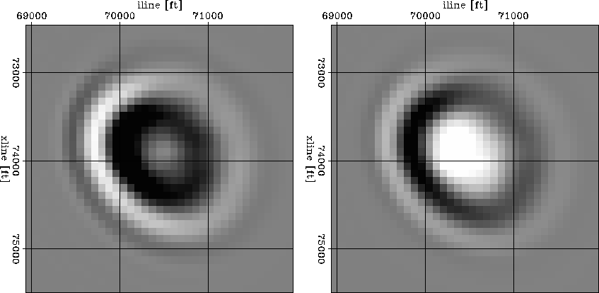
Figure 15 Cross-section of 3D sensitivity kernels for wave-equation MVA. The left panel corresponds to an image perturbation produced a kinematic shift, while the right panel corresponds to an image perturbation produced by amplitude scaling. The lowest sensitivity occurs in the center of the kinematic kernel (left). In contrast, the maximum sensitivity occurs in the center of the kernel (right).

frechet.exp can be written formally as  

$$\delta \dat= {\bf F}_0\delta \mod\;,$$ (72)

where $\delta \mod$ is a perturbation in the model space, and $\delta \dat$ is a perturbation in the image space. If we denote by $\delta d^i$ the i^th component of $\delta \dat$, and by $\delta \mod\lp \xx \rp$ an infinitesimal element of $\delta \mod$at location $\xx$, we can write  

$$\delta d^i= \int_V F_0^i\lp \xx \rp\; \delta \mod\lp \xx \rp\; dv\lp \xx \rp\;.$$ (73)

F₀ⁱ is, by definition, the integral kernel of the Fréchet derivative ${\bf F}_0$,V is the volume under investigation, dv is a volume element of V and $\xx$ is the integration variable over V. The sensitivity kernel, a.k.a. Fréchet derivative kernel , F₀ⁱ expresses the sensitivity of $\delta d^i$ to a perturbation of $\delta \mod\lp \xx \rp$ for an arbitrary location $\xx$ in the volume V.

Sensitivity kernels occur in every inverse problem and have different meanings depending of the physical quantities involved:

For wideband traveltime tomography (104; 14; 3; 33; 55), $\delta \dat$ is represented by traveltime differences between recorded and computed traveltimes in a reference medium. The sensitivity kernels are infinitely-thin rays computed by ray tracing in the background medium. For finite-frequency traveltime tomography (28; 52; 58; 76), $\delta \dat$ is represented by time shifts measured by crosscorelation between the recorded wavefield and a wavefield computed in a reference medium. The sensitivity kernels are represented by hollow fat rays (a.k.a. ``banana-doughnuts'') which depend on the background medium. For wave-equation tomography (114; 72; 73), $\delta \dat$ is represented by perturbations between the recorded wavefield and the computed wavefield in a reference medium. The sensitivity kernels are represented by fat rays with similar forms for either the Born or Rytov approximation. For wave-equation migration velocity analysis (10; 88; 89; 93), $\delta \dat$ is represented by image perturbations. The sensitivity kernels are discussed in the following sections.

Wave-equation migration velocity analysis (WEMVA) establishes a linear relation between perturbations of the slowness model $\DEL s$ and perturbations of migrated images $\DEL \RR$.$\DEL s$ and $\DEL \RR$ correspond, respectively, to $\delta \mod$ and $\delta \dat$ in linear.

Formally, we can write

$$\Delta \RR= \Lop \Delta s\;,$$ (74)

where $\Lop$ is the linear first-order Born wave-equation MVA operator. The operator $\Lop$ incorporates all first-order scattering and extrapolation effects for media of arbitrary complexity. The major difference between WEMVA and wave-equation tomography is that $\delta \dat$ is formulated in the image space for the former as opposed to the data space for the later. Thus, with WEMVA we are able to exploit the power of residual migration in perturbing migrated images - a goal which is much harder to achieve in the space of the recorded data.

By construction, the linear operator $\Lop$ depends on the wavefield computed by extrapolation of the surface data using the background slowness, which corresponds to $\mod_0$ in frechet.exp. Thus, the operator $\Lop$ depends directly on the type of recorded data and its frequency content, and it also depends on the background slowness model. Thus, the main elements that control the shape of the sensitivity kernels are

the frequency content of the background wavefield, the type of source from which we generate the background wavefield (e.g. point source, plane wave), and the type of perturbation introduced in the image space, which for this problem corresponds to the data space.

In the next examples, I define two types of image perturbations: a purely kinematic type $\DEL \RR_k$, implemented simply as a derivative of the image with respect to depth, which can be implemented as a multiplication in the depth domain as follows:  

$$\DEL \RR_k = -i \zz \widetilde{\RR}\;,$$ (75)

and a purely dynamic type $\DEL \RR_a$, implemented by scaling the reference image $\widetilde{\RR}$ with an arbitrary number:  

$$\DEL \RR_a = \epsilon \widetilde{\RR}\;.$$ (76)

In both cases, the perturbations are limited to a small portion of the image. The main difference between $\DEL \RR_k$ and $\DEL \RR_a$is given by the $90^\circ$ phase-shift between the two image perturbations.