


Next: WEMVA operator
Up: Wave-equation migration velocity analysis
Previous: Recursive wavefield extrapolation
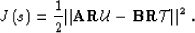
Migration velocity analysis is based on estimating the velocity
that optimizes certain properties of the migrated images.
In general, measuring such properties involves making
a transformation after wavefield extrapolation to the migrated
image using a generic differentiation function  characterizing image imperfections
|  |
(56) |
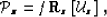
where  is the imaging operator applied to the
extrapolated wavefield
is the imaging operator applied to the
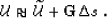
extrapolated wavefield  .In compact matrix form, we can write this relation as:
|  |
(57) |
The image  is subject to optimization from
which we derive the velocity updates.
is subject to optimization from
which we derive the velocity updates.
Two examples of transformation functions are:
 where
u denotes an extrapolated wavefield and
where
u denotes an extrapolated wavefield and
 is a known target wavefield.
A WEMVA method based on this criterion optimizes
is a known target wavefield.
A WEMVA method based on this criterion optimizes
|  |
(58) |
where  stands for the target wavefield.
For this method, we can use the acronym TIF
standing for target image fitting
(10; 88; 89; 93).
stands for the target wavefield.
For this method, we can use the acronym TIF
standing for target image fitting
(10; 88; 89; 93).
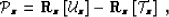
 where
where  is a known operator.
A WEMVA method based on this criterion optimizes
is a known operator.
A WEMVA method based on this criterion optimizes
|  |
(59) |
If is a differential semblance operator,
we can use the acronym DSO standing for
differential semblance optimization
(105; 97).
In general, such transformations belong to a
family of affine functions that can be written as
|  |
(60) |
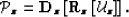
or in compact matrix form as
|  |
(61) |
where the operators  and
and  are known and
take special forms depending on the optimization criterion we
use. For example,
are known and
take special forms depending on the optimization criterion we
use. For example,  and
and  for TIF,
and
for TIF,
and  and
and  for DSO.
 stands for the identity operator, and
 stands for the null operator.
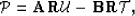
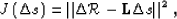
With the definition in affine.z, we
can write the objective function J as:
Js
&=& 12_,m,h || ||^2
stands for the null operator.
With the definition in affine.z, we
can write the objective function J as:
Js
&=& 12_,m,h || ||^2
&=& 12_,m,h || _z_z- _z_z||^2 ,
where s is the slowness function, and
 stand respectively for depth, and the midpoint and
offset vectors.
In compact matrix form, we can write the objective function as:
stand respectively for depth, and the midpoint and
offset vectors.
In compact matrix form, we can write the objective function as:
|  |
(62) |
In the Born approximation,
the total wavefield is related to the background wavefield  by the linear relation
|  |
(63) |
If we can replace the total wavefield in the
objective function objective, we obtain
| 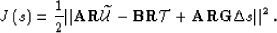 |
(64) |
objective.linear describes a linear optimization problem,
where we obtain  by minimizing the objective function
|  |
(65) |
where 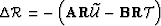 , and
, and
 .The operator
  is constructed based on the
Born approximation (56),
and involves the pre-computed background wavefield through the
background medium.
A discussion on the implementation details
for operator is presented in Appendix C.
The convex optimization problem defined by the linearization in
objective.linear can be solved using standard
conjugate-gradient techniques.
is constructed based on the
Born approximation (56),
and involves the pre-computed background wavefield through the
background medium.
A discussion on the implementation details
for operator is presented in Appendix C.
The convex optimization problem defined by the linearization in
objective.linear can be solved using standard
conjugate-gradient techniques.
Since, in most practical cases, the inversion problem
is not well conditioned, we need to add constraints on the
slowness model via a regularization operator.
In these situations, we use the modified objective
function
|  |
(66) |
Here,  is a regularization operator,
 is a weighting operator on the data residual, and
 is a scalar parameter which balances
the relative importance
of the data residual (
is a scalar parameter which balances
the relative importance
of the data residual (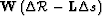 ) and
of the model residual (
) and
of the model residual ( ).
).
Next: WEMVA operator
Up: Wave-equation migration velocity analysis
Previous: Recursive wavefield extrapolation
Stanford Exploration Project
11/4/2004